Last year, we simulated the Underdog Best Ball Mania IV Finals for Week 17. We ran the simulations after the Thursday night game and then again after Saturday night’s games. It was fun to track and provide the contestants with some sweat material.
Fast forward a few months later, and we revisited those simulations to try and glean some characteristics about the makeup of the finals. In many ways, using our simulations in lieu of the actual results is a more informative way of analyzing the best teams in the Week 17 finals, since it captures the full range of outcomes of what could have happened — not just one static result. Of course, it’s impossible for these simulations to be perfect, and they reflect the bias of the ETR projections for that week.
The only change we made in simulating the Week 17 Finals is applying the *current* Best Ball Mania’s payout structure, which is much flatter than last season’s payout structure was. Of course, there weren’t as many contestants in the finals last year (441 to this year’s 539), so the EV is somewhat inflated for each team, but this gives us more actionable information to consider when drafting now.
This is a mostly descriptive exercise. While many of the findings are quite interesting to me (and hopefully to you as well!), it’s important to remember that pod variance in dictating the finalists, health of teams, and the season only playing out one actual way (rather than the millions of iterations it could have played out) are an overwhelming factor here, even if our simulations allow us to cover a more full range of outcomes for the finals week specifically.
In the coming weeks, I hope to do a rehashed version of last year’s Best Ball Mania Manifesto, which should shed a broader light on the importance of stacking, ADP value, and roster construction, but this one-week view at the simulated finals is a nice complement to the Manifesto, which may not properly fully correlate the results of an estimated finals week to the results of an actual finals week.
Below, I’ll look at the average EV (expected value), Win Rate, and Top-10 rate of groups of teams based on number of live players, stacking, ADP value, and positional allocations. Where relevant, I’ll first look at how frequently teams of a certain characteristic made the finals relative to how likely any team (677,376) or any playoff team (112,896) was to have the same characteristic. For example, if 46% of the finals teams drafted three QBs but only 40% of all teams drafted three QBs, we know these teams performed better than expected by about 15% in terms of ability to make it to the finals.
Leaderboard
Here is a Google Sheet link to the full field Simulated Expected Value as well as odds of winning the tournament and odds of finishing top 10: https://docs.google.com/spreadsheets/d/13ksEqGbq0ptdwjmFGOCdezzkF302jIkTnOLkozpNVSM/edit?usp=sharing.
Stacking
I wanted to start with stacking because it’s such a critical component of winning best ball tournaments, especially those with a playoff structure like Best Ball Mania’s. The stacking section will also provide us a lesson on trying to discern “the best strategies” from “the most common strategies the best players use”. That might sound like semantics, but it’s an important distinction.
Field Utilization
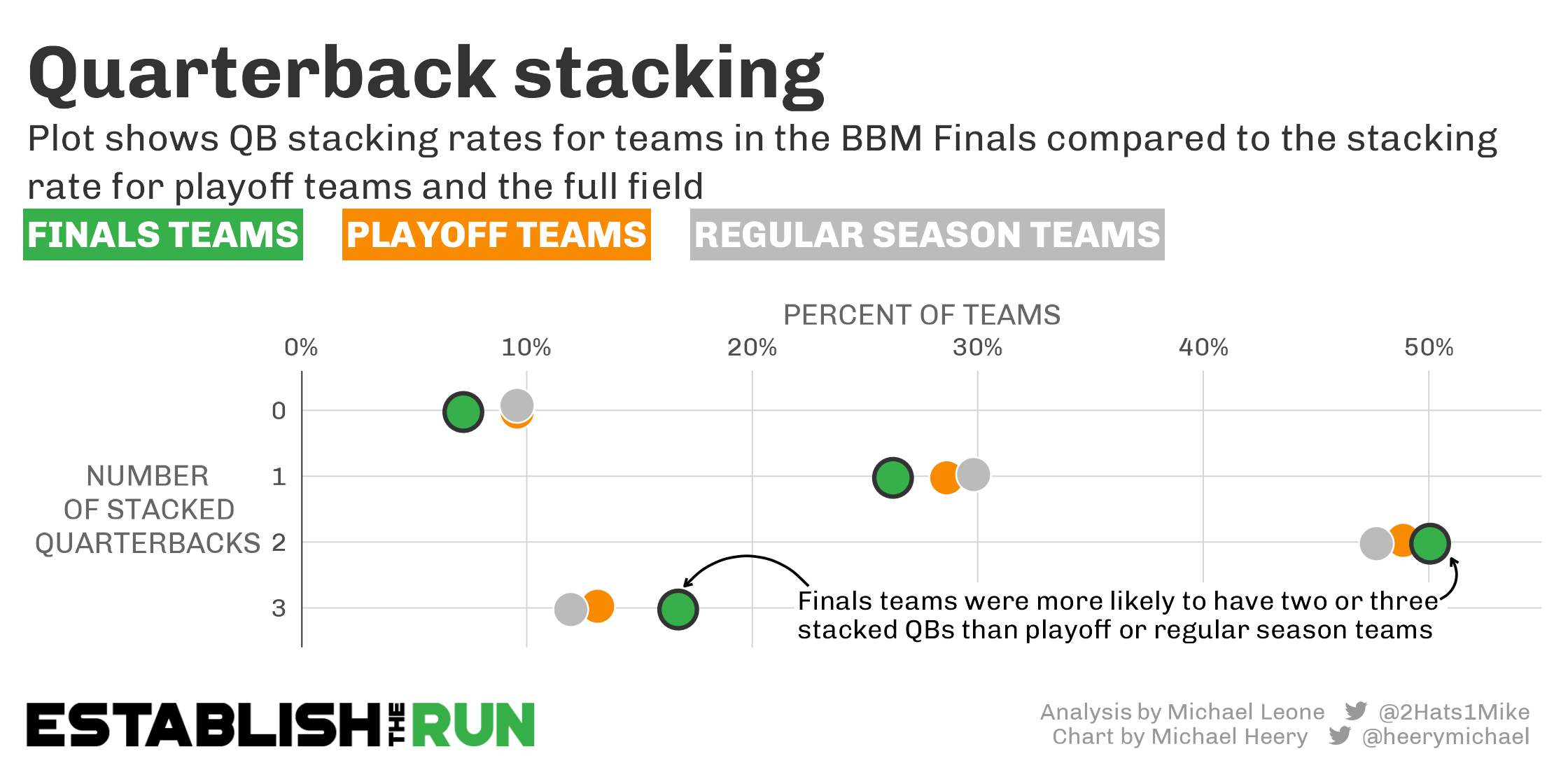
Teams that stacked (rostered a QB with one of their pass catchers) more heavily made up a higher percentage of the finals field than they did all teams drafted or playoff teams in particular. The comparison to all playoff teams is particularly apt, as it likely shows that stacked teams had better odds of winning a weekly Underdog playoff pod than those with less stacking.
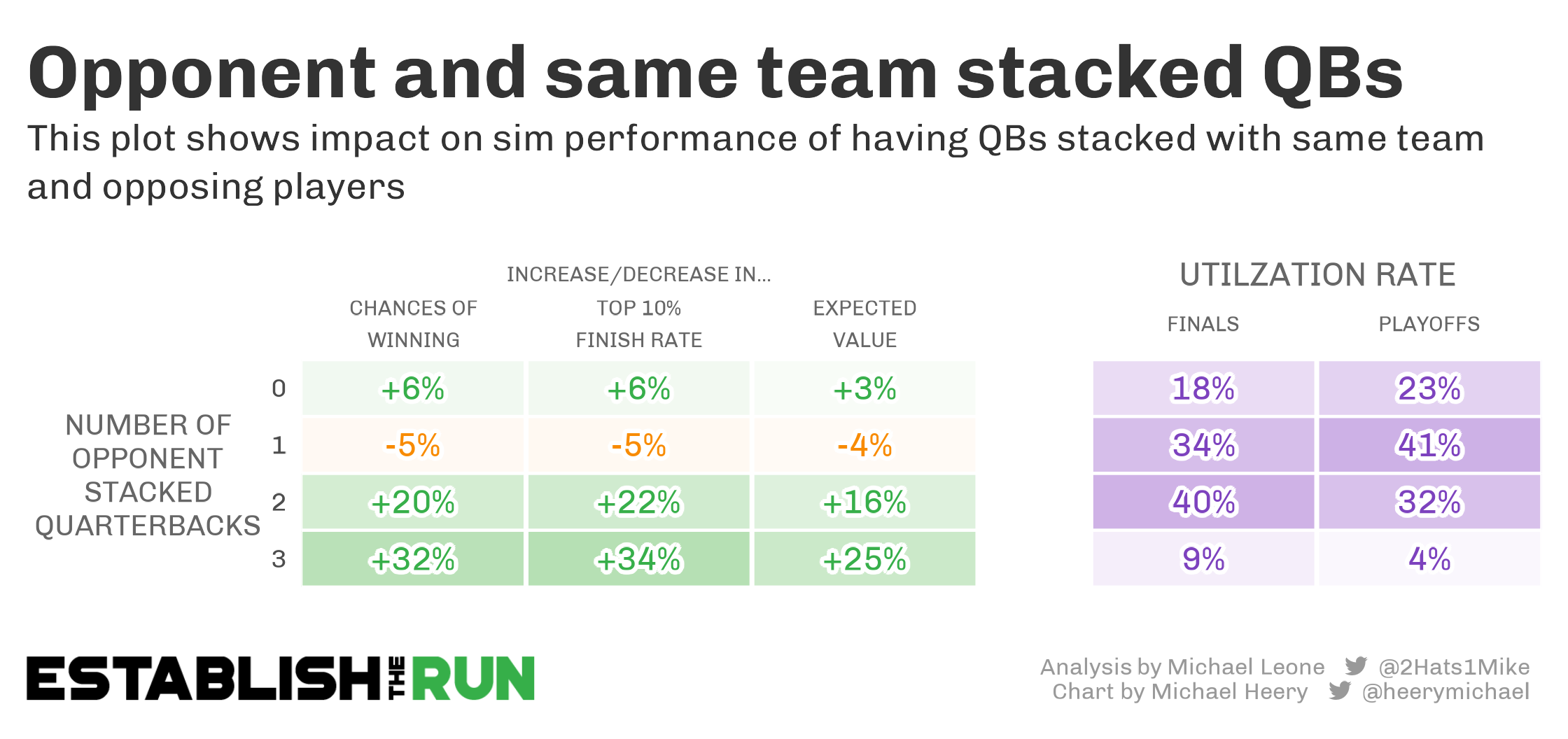
Teams with three stacked QBs were 23% more likely than random to make it to the finals, while teams with zero stacked QBs were 26% less likely.
An interesting wrinkle, though, is that teams with more Week 17 QBs game stacked had their odds increase quite a bit further beyond expectation. A game stack is considered a stacked QB from above plus at least one opponent skill player for that specific week.
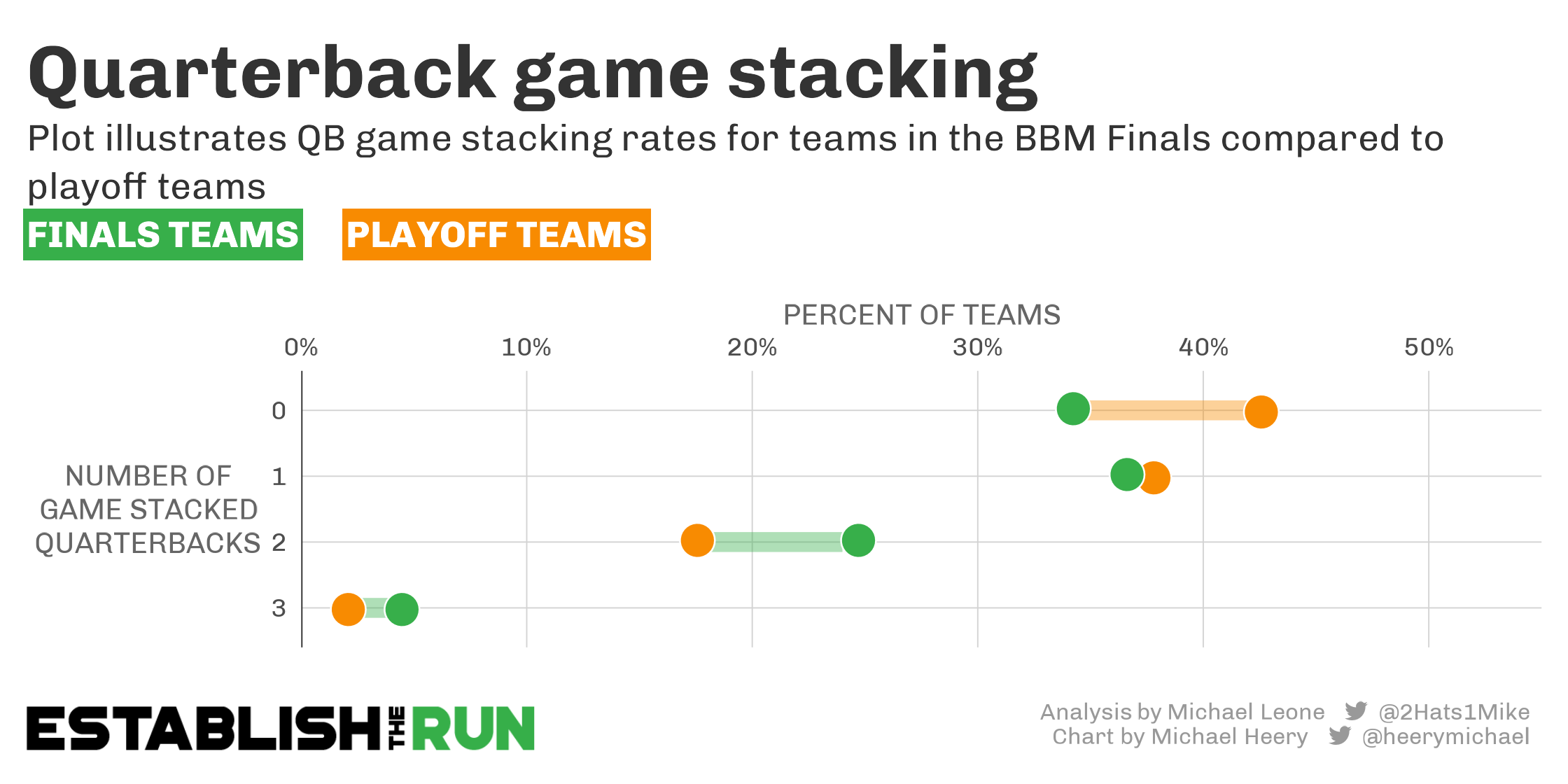
In one sense, this is logical. You can’t have a game stack without first having a regular stack, and we just showed the teams with three stacked QBs were 23% more likely to make it to the finals than their overall playoff representation would indicate.
On the other end, this makes no sense at all. Week 17 game stacking should increase a team’s odds of performing well in Week 17, not in Weeks 15 and 16. There should not be any correlation (beyond that of regular stacking) tying Week 17-specific game stacks to increased finals participation rate.
The only explanation for this in my eyes is this: Sharper players are setting up Week 17 game stacks more than the average player. So what this data tells is not that stacking Week 17 increases your odds of making it to the finals once you reach the playoffs, but that sharper players are drafting better teams and more likely to make it to the finals once they reach the playoffs.
This is an important meta to keep in mind when evaluating any past, descriptive data. I think it likely has an impact on the success of Zero RB for example. It’s not that these strategies aren’t sharp, but it’s difficult to discern at times how much of the success of the strategy is coming from the strategy itself or the skill of the drafters employing the strategy.
Here’s another view of the dynamic I am talking about. In order to strip out any potential bias in heavy game stacking teams necessarily being heavily team stacked in the first place, I looked at only playoff teams and finals teams where every QB rostered was team stacked.
As you can see, even in this subset the teams that rostered bring-backs in Week 17 were more likely to make it to the finals than those that didn’t. This provides further evidence that, on the whole, users who Week 17 game stacked had better teams than those that didn’t — for reasons that had nothing to do with Week 17 game stacking.
Removing the meta itself, this strategy also fulfilled its intent — increasing Expected Value once you make the finals. Teams with all of their QBs team stacked saw big improvements in simulated Week 17 Expected Value when they also drafted a bring-back for two or three of their QBs.
Putting all of this context together, I have two key takeaways:
- Week 17 game stacking is +EV
- You can build Week 17 game stacks without sacrificing your ability to make it to Week 17
Let’s dive a bit more into Expected Value based on stacking tendencies among the Week 17 finalists.
Week 17 Expected Value
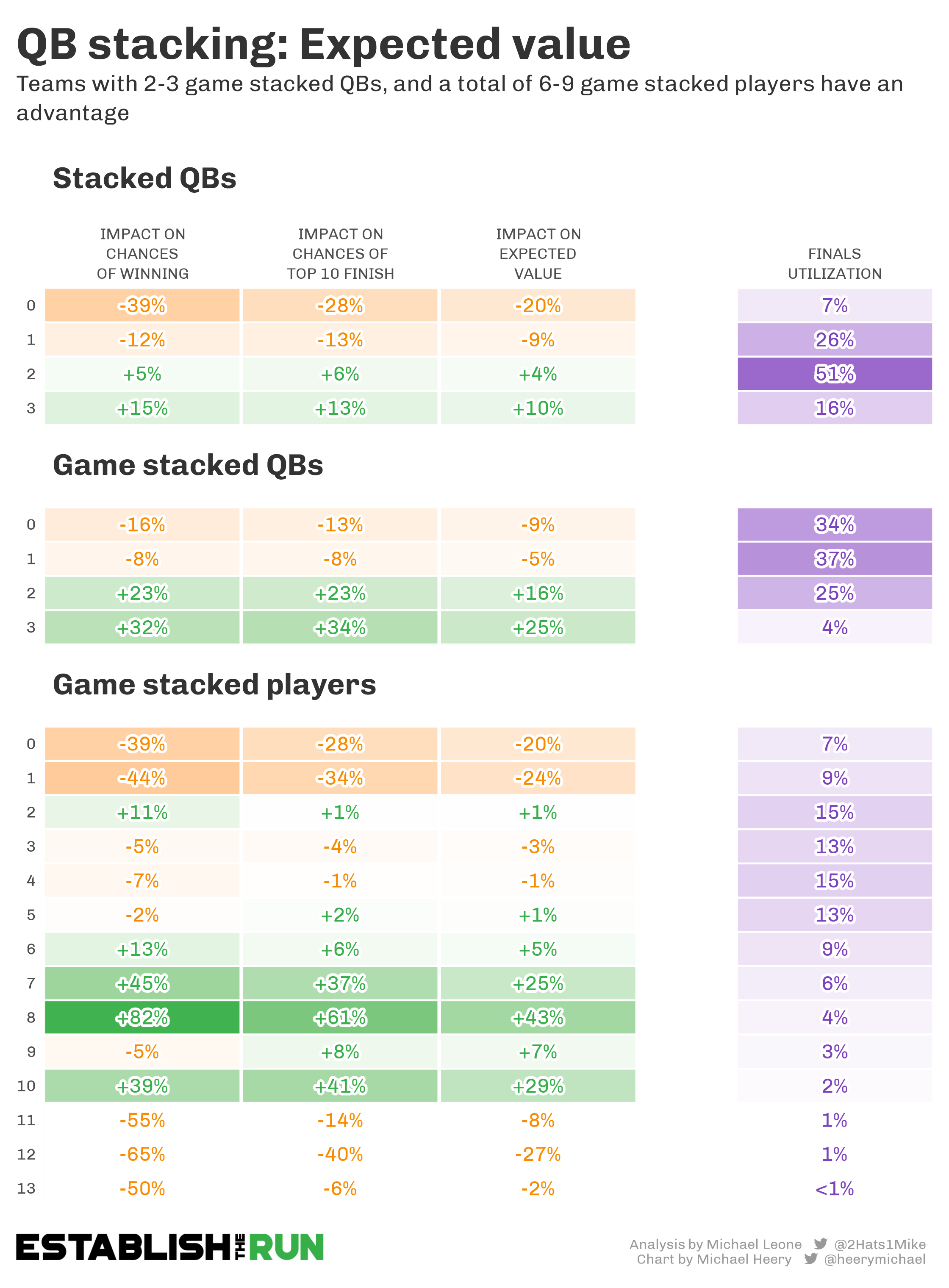
Key Notes:
- Teams with 0 or 1 team-stacked QB are operating at a serious disadvantage.
- Teams with 2 or 3 game-stacked QBs are operating at a serious advantage.
- From last year’s Manifesto, we pegged 6-9 game-stacked players as the range to target when building teams. In last year’s actual finals, teams with 6-10 game-stacked players had the highest average EV of any cohort, but just 15% of W17 finalists did this.
- 11+ game-stacked players is probably too many. 0-1 game-stacked players is way too few. 2-5 game-stacked players puts you at mostly a neutral expectation.
Live Players
One of the most important facets of competing in a Week 17 final is, to a large extent, outside of our control — how healthy are our players, and do they have any sort of role on a depth chart? To measure this, I looked at the number of “live” players on each team and how that impacted a team’s Expected Value. A “live” player is any player who scored more than zero fantasy points in the week.
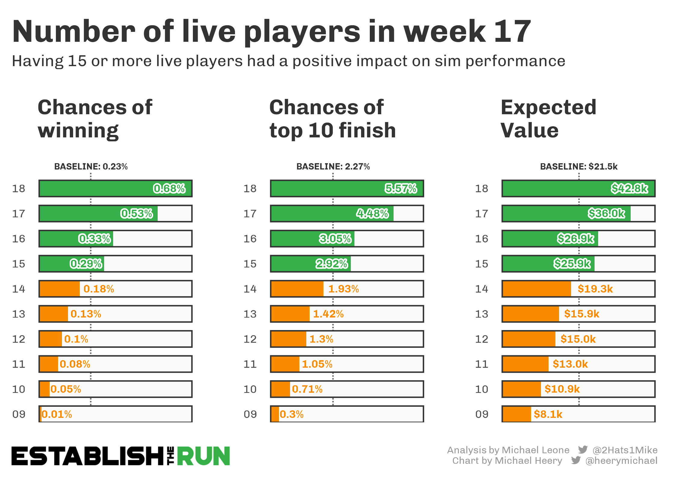
This image paints a stark reality. Less than 14 live players in Week 17 almost cuts your Expected Value in half. More than 14 live players in Week 17 almost doubles your Expected Value.
It’s not up to debate how important it is to simply have a full roster of possibly contributing players on your roster in Week 17. What is up for debate is if you can control this at all, and if so, how? I touched on this to some extent in last year’s Manifesto, but my subjective takeaways are to draft mid-July or later and have a healthy balance of younger players who can ascend and established players with defined roles on your roster.
I thought perhaps that taking three late-QBs, which already has additional game stacking benefits for Week 17, would also increase your odds of having live players late in the season. The idea is that QBs late have more job security than RBs and WRs, but the actual data only bears this out very mildly.
ADP Value
Before diving into the importance of ADP value, let’s do a quick refresher in how I am viewing ADP value. I assigned each draft spot a certain amount of “draft capital” based on a model linking points contributed to best ball roster above positional average to draft spot.
Based on this model, pick 10 is worth 117.9 points of “draft capital”, while pick 5 is worth 124.0 points. So if you drafted a player with an ADP of 5 with the 10th overall pick, you’d gain 6.1 points of draft capital (ADP Capital – Pick Capital, 124.0 – 117.9 = 6.1).
For the full breakdown of what draft capital I am assuming for each pick, you can check out this Google Sheet: https://docs.google.com/spreadsheets/d/1znGWgHPVQH5nmHcpKVJzR0GcTPTdI-PmjMO9NP92EzM/edit?usp=sharing.
This is how I am determining ADP value. I am then breaking teams down into 10 equal buckets based on their total ADP value for their roster. If a team is in Bucket 1, they are among the top 10% of teams in total ADP value. If a team is in Bucket 10, they are among the bottom 10% of teams in total ADP value.
Closing line ADP value is determined using a player’s final ADP. Real time ADP value is determined using a player’s ADP that was seen in the draft room at the time they were selected.
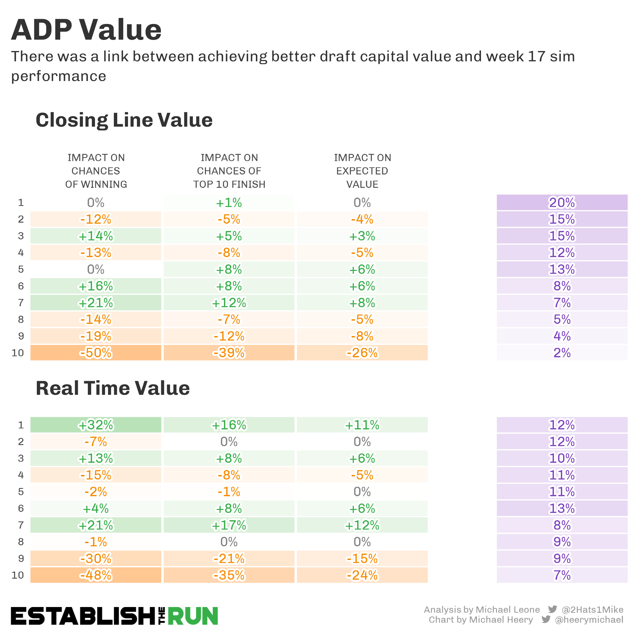
One of the best ways to build super teams is to compile a bunch of closing line ADP Value. Teams in the top 10% made the finals at a rate nearly double that of randomness. The first five buckets of closing line ADP value were all overrepresented among finalists, while the last five buckets were all underrepresented.
The most stark changes in expectation occurred:
- Positively for Bucket 1 Teams
- Negatively for Bucket 8, 9, and 10 teams
The effects were much more muted in terms of real time ADP value. The top six buckets were all overrepresented while the bottom four buckets were all underrepresented, but the correlation was much smaller.
You might think that any ADP value, closing or real time, would cease to matter among the specific subset of teams that made the Week 17 finals, but there was still a link between better ADP value and Week 17 Expected Value among the finalists. This is most clear at the bottom end: Buckets 8, 9, and 10 from both closing and real time ADP value all had a below-average EV in Week 17.
If you’re building solely with Week 17 in mind, it’s obvious that stacking trumps ADP value. A neutral team in terms of ADP value with lots of correlation is way more valuable than one of the best teams in terms of ADP value but with very little correlation. Just make sure you avoid being in a Bottom 3 bucket.
Roster Construction
Quarterback
Utilization
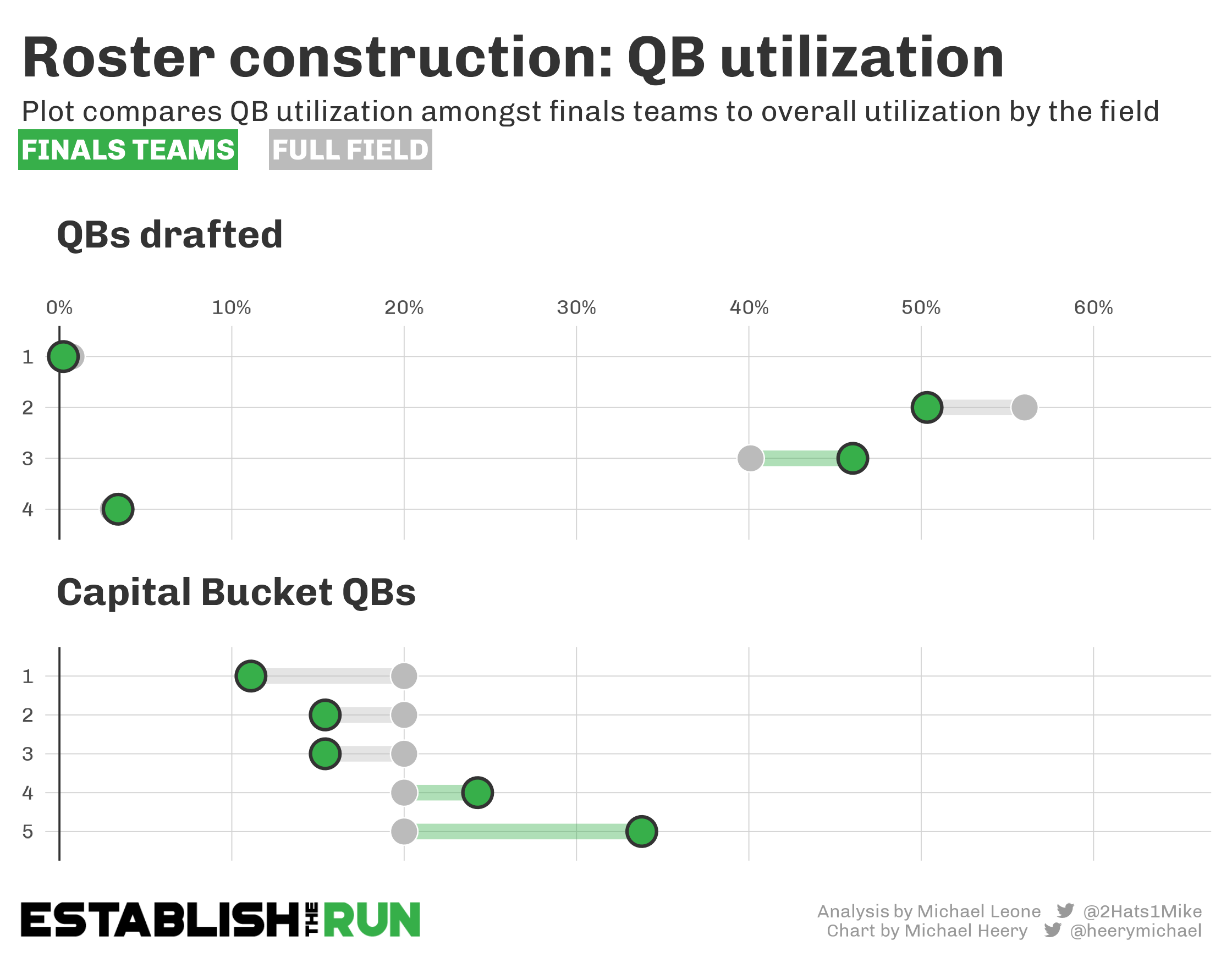
Key Notes:
- Three QBs appeared in the finals at a higher rate than expected.
- Connected to that, the less capital you spent at the position, the more likely you were to make the finals (and these teams were more likely to roster three QBs late).
- It was a bad year in the aggregate for elite QBs.
Finals EV
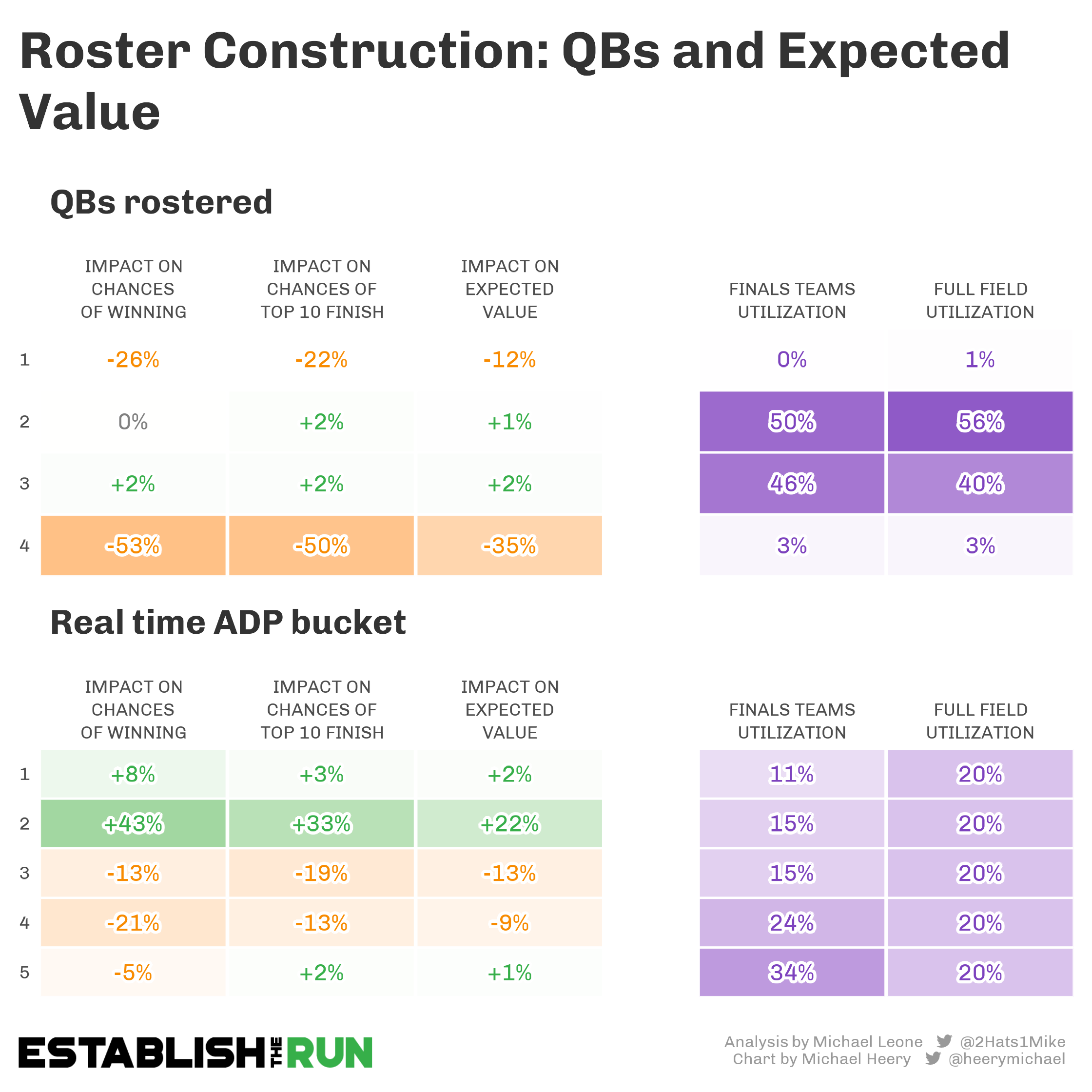
Key Notes:
- Two or three QBs remains optimal — no need to get fancy.
- Teams with higher-end QB teams had a hard time making it to finals but held more win equity in Week 17.
Wide Receiver
Utilization
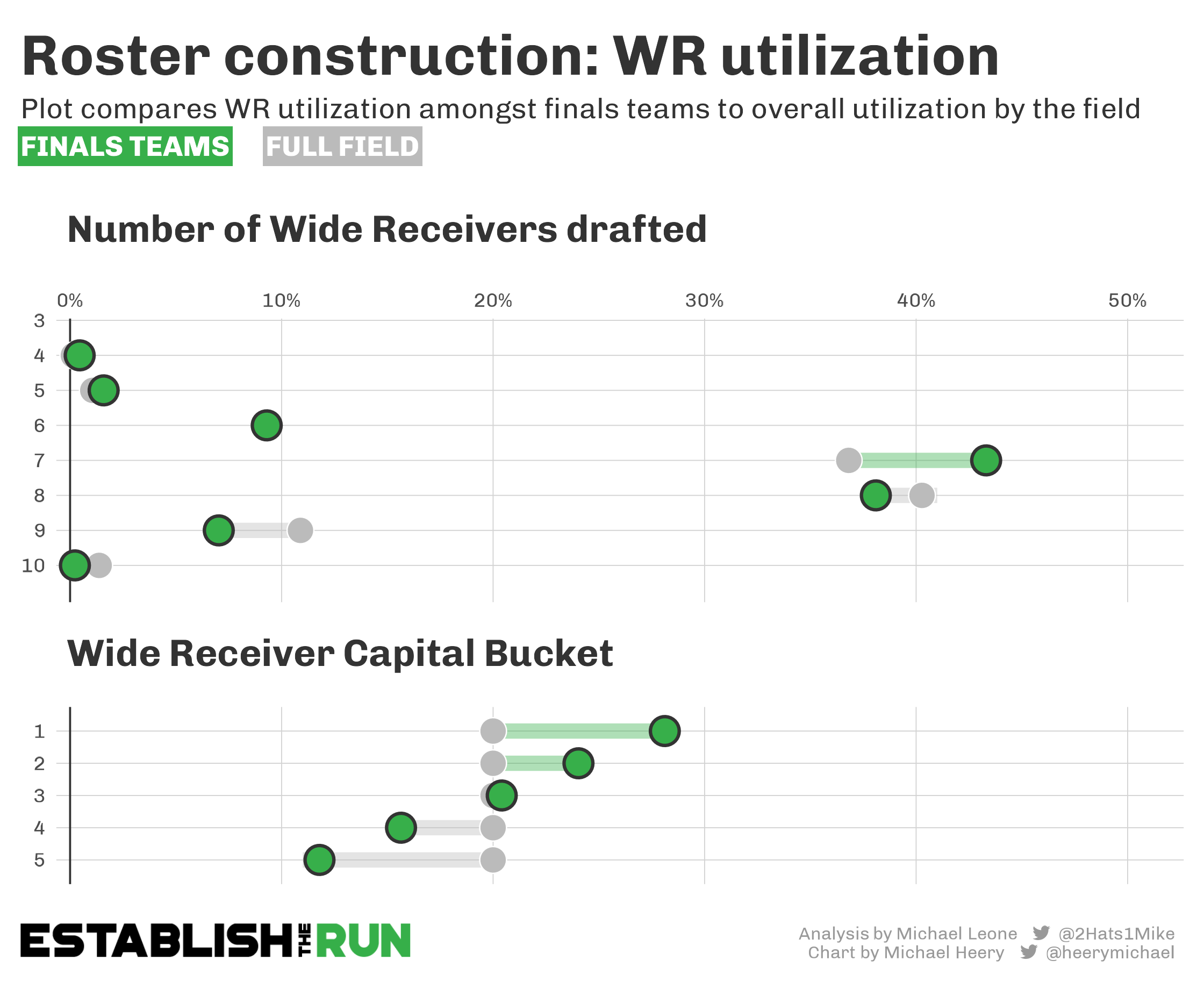
Key Notes:
- Teams that spent more capital at WR were largely overrepresented and vice versa.
- The leverage of 4- and 5-WR teams is overstated due to the small sample, but it is clear that you don’t need to be drafting 8+ WRs, especially when investing early.
Expected Value
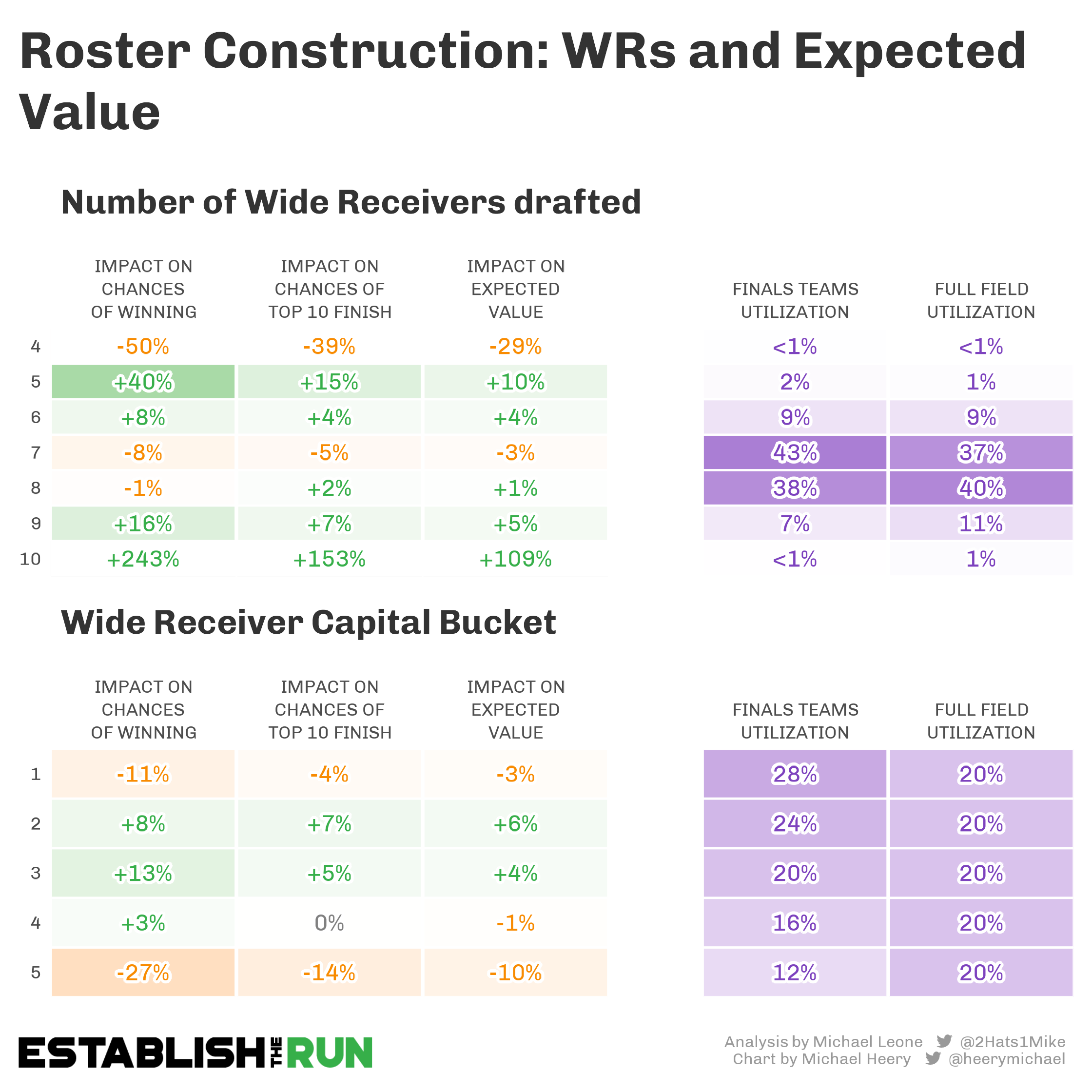
Key Notes:
- Capital at the WR position was not quite as important once you made the finals, as long as you weren’t in the fifth bucket.
- Likewise, the quantity of WRs was also less important in Week 17 itself.
Running Back
Utilization
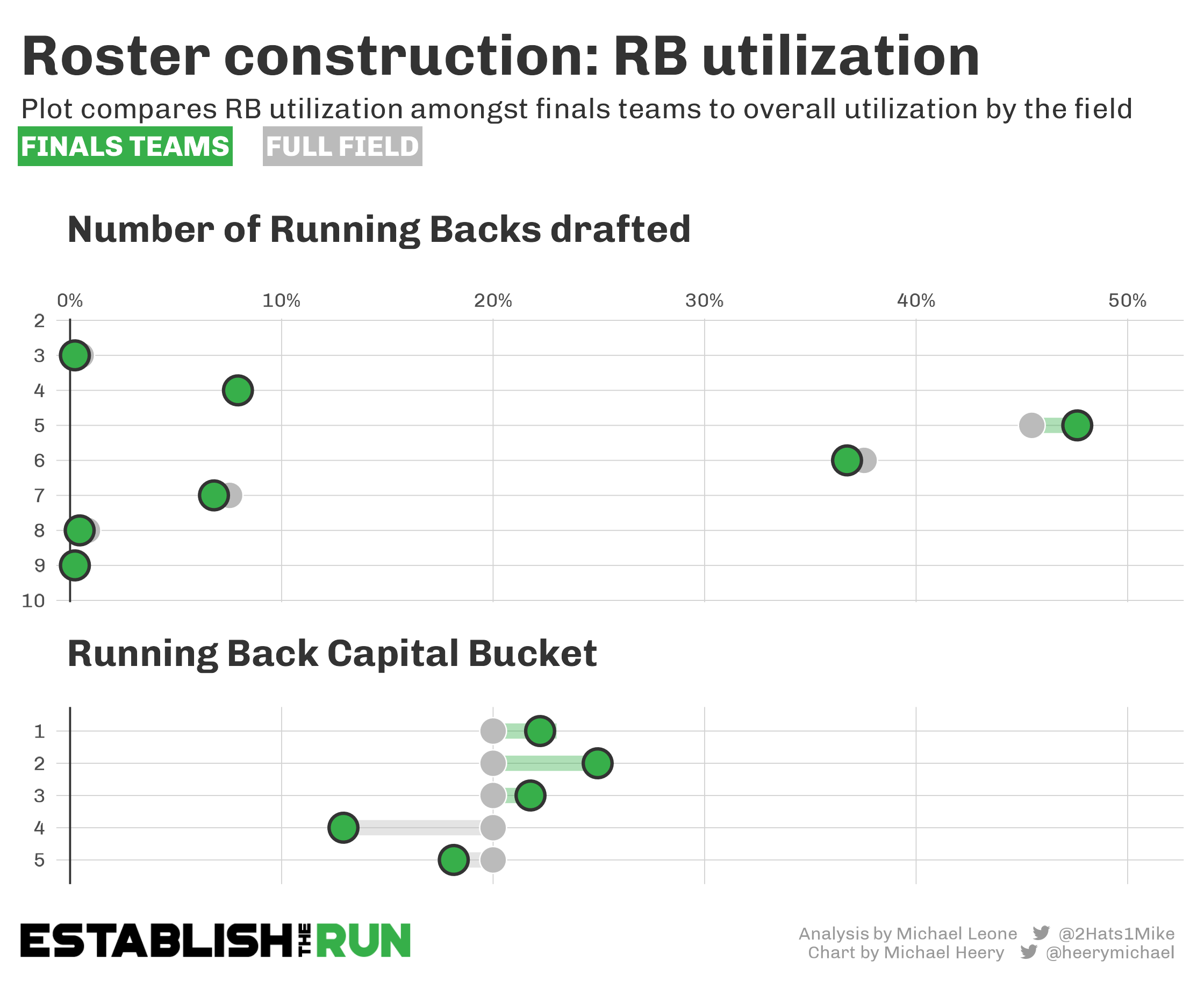
Key Notes:
- Teams that drafted 6+ RBs were a little bit underrepresented in the finals.
- Teams that drafted 4-5 RBs were a little bit overrepresented in the finals.
- Teams in the top three RB capital buckets were overrepresented in the finals, while teams in the bottom two buckets were underrepresented.
Expected Value
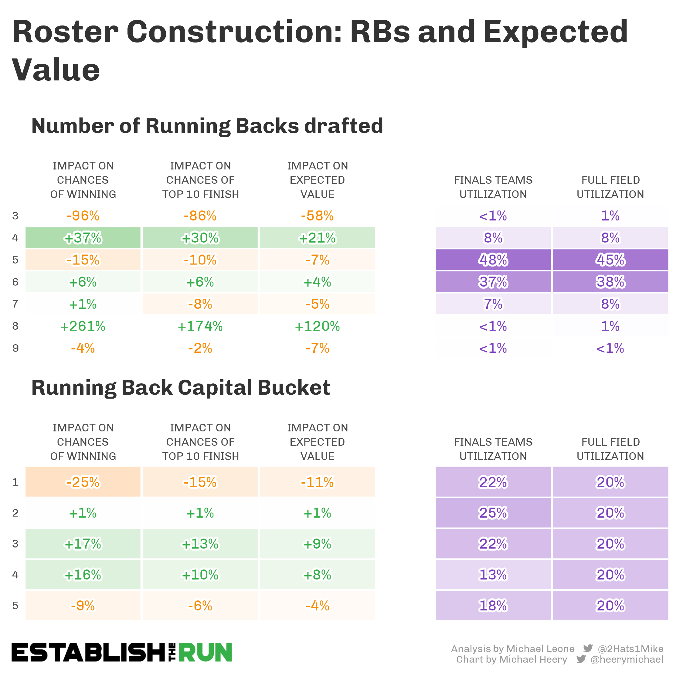
Key Notes:
- 4-RB teams had the highest EV among builds with a sample size greater than 10 in the finals (more on that below).
- Otherwise, EV spread among the quantity of RBs rostered was fairly flat.
- Teams that had a middle amount of investment in the RB position (capital buckets 2-4) performed the best in Week 17 in terms of Win rate, Top-10 rate, and overall EV.
It’s interesting that hyperfragile teams made it to the top of some of our highest Best Ball Mania III simulated EV teams in last year’s Manifesto, despite the models being entirely trained on a year’s worth of data where those teams en masse did not perform well.
This season, we see that these teams performed just okay in Best Ball Mania IV given their neutral representation in the finals. Yet, the teams that made it to the finals with this type of build were very +EV in Week 17 itself. Pat Kerrane also won Best Ball Mania III with a hyperfragile build.
My point here is not to ignore the aggregate data. You clearly do not want to be building a lot of hyperfragile RB teams. However, you don’t want to blanket remove the strategy from your toolbox simply because it did not perform well overall, especially if you’re willing to adapt the strategy to fit the current draft landscape.
One thing that’s clear from last year’s Manifesto and analyzing these finals is that the strength of a team is based on the complex makeup of all of its characteristics: correlation, value, proper positional allocation based on how you start, etc.
As a result, I like to keep in mind these broader +EV strategies but ultimately be willing to be quite flexible within a draft itself, trusting myself to put the pieces of the puzzle together well and tie it together by the end.
A closer look at the combination of quantity of RBs chosen with total RB capital invested shows that hyperfragile teams in any bucket had the potential to perform well. Meanwhile, teams that drafted a high quantity of RBs wanted to avoid investing a lot of overall capital into the position.
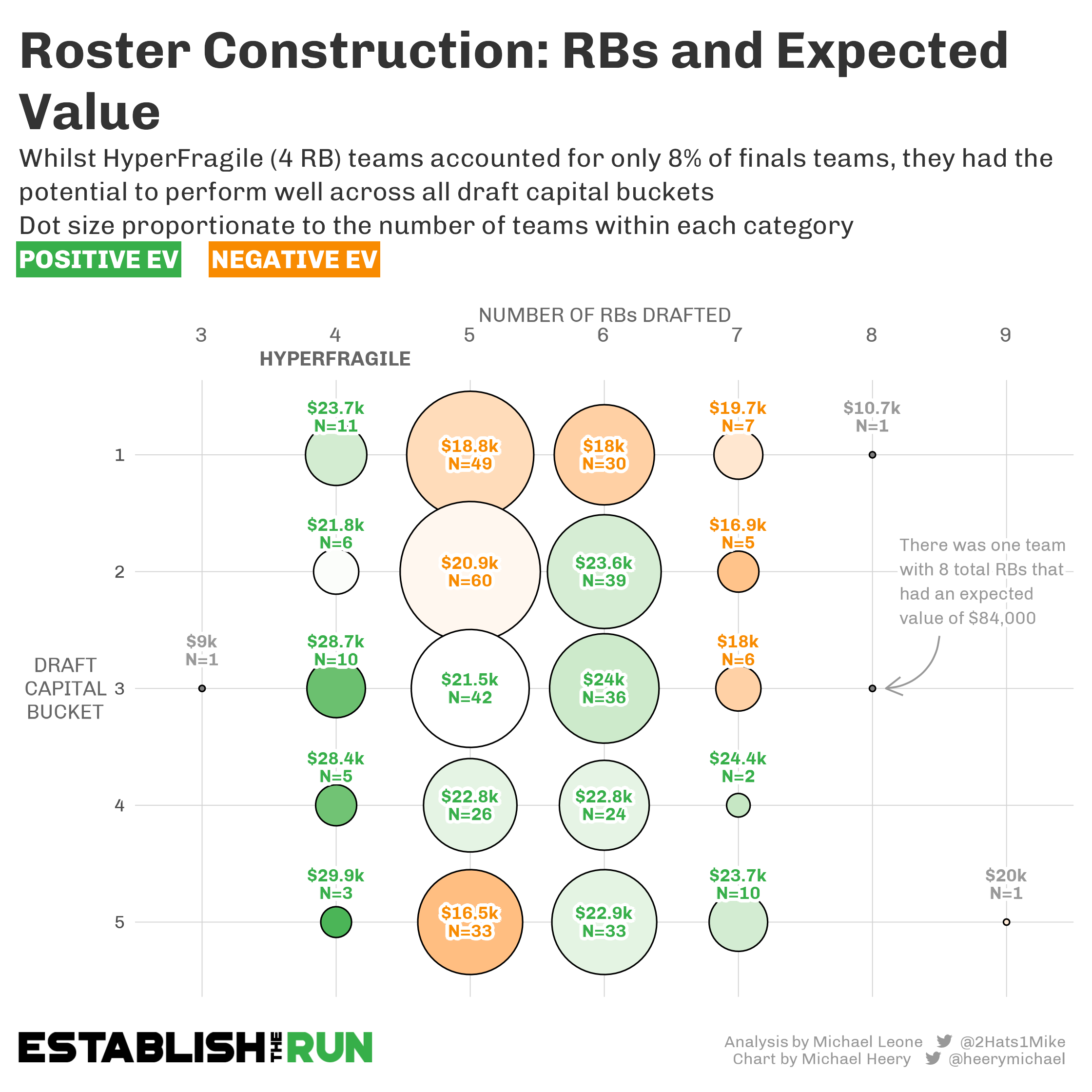
Unlike when I first wrote about hyperfragile RB teams, you do not want to be drafting three to four RBs early. The WR landscape has changed too much. It’s harder than ever to beat quantity with quality in that position as the ADPs of the position get pushed up en masse.
The best 4-RB teams in the Week 17 finals last season were either CMC teams that drafted one or two mid to high single-digit-round RBs, or teams that paired Breece Hall with Jahmyr Gibbs (Rounds 3 and 4) and took one other mid to late single-digit-round RB. Almost all of these builds had the fourth and final RB drafted in the double-digit rounds.
If drafting hyperfragile teams in Best Ball Mania V, I’d adopt a similar construction (one or two RBs in the first five to six rounds, two or three more RBs in Rounds 7 through 14ish), which enables you to still keep up at WR in terms of quality early. In some cases, you can even sneak in an elite onesie and still technically be on the hyperfragile track. I’d be fine extending four RBs to five RBs since the capital you’re investing in RB still isn’t heavy for the group in totality.
Tight End
Utilization
Key Notes:
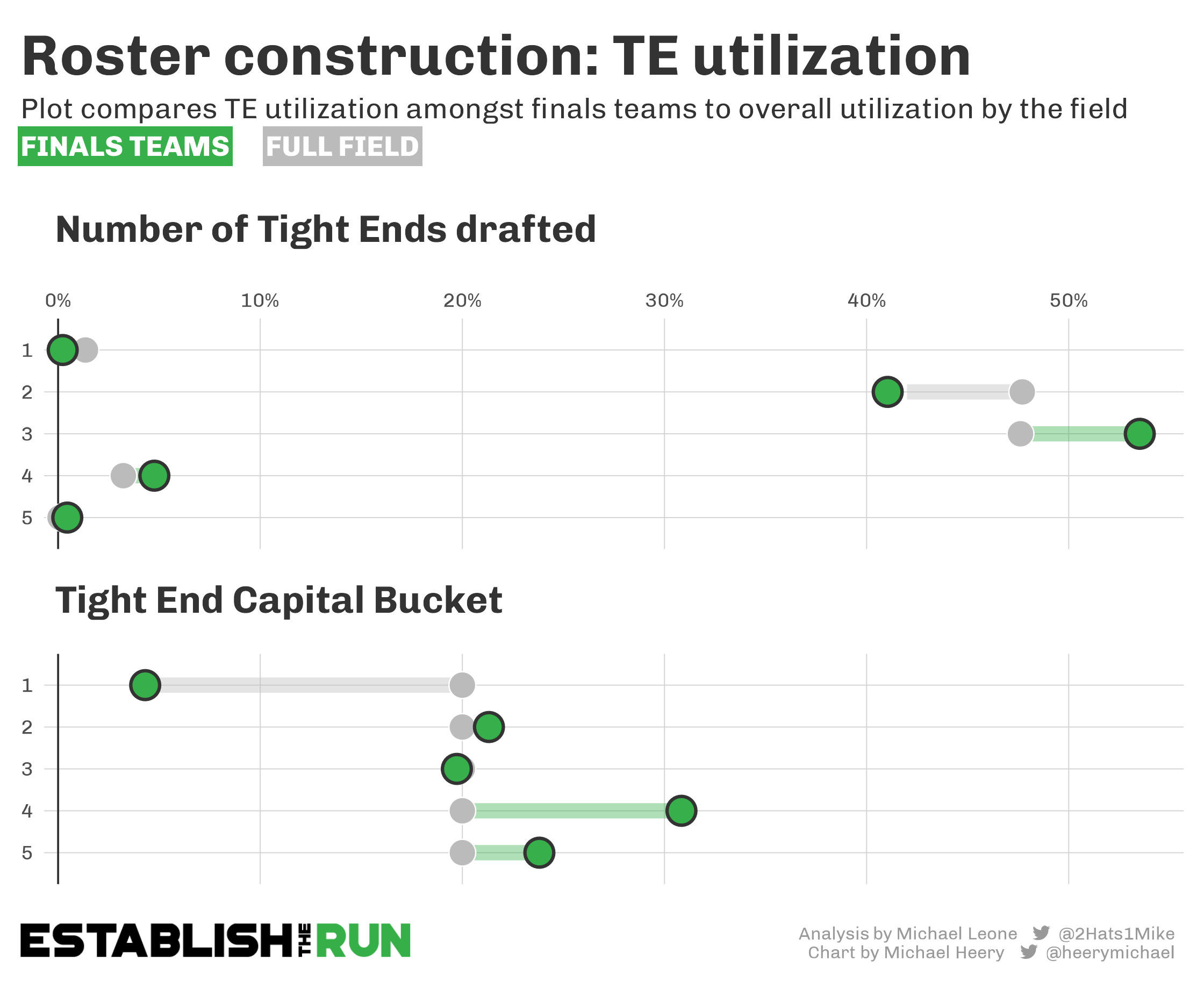
- 3-4 TE teams (technically five too, but would not recommend it) were overrepresented while 1-2 TE teams were underrepresented.
- Teams investing a lot of capital in TE (Bucket 1) had a very poor finals advance rate, while Buckets 5 and particularly 4 exceeded expectations.
The TE position is a good spot to point out how a lot of this wraps together. WR Buckets 1-3 performed well and, to a lesser extent, so did RB Buckets 1-3. It’s not surprising this aligns with a down year at QB and TE where investing in the elites at either onesie position by and large did not pay off. So, was it more important to invest in RB and WR early, or was it more important to avoid the early QB and TE landmines?
It’s also worth noting that the spike in TE Bucket 4 being overrepresented in the finals has a lot to do with where Sam LaPorta was drafted, as he was one of the highest-owned players in the finals.
Expected Value
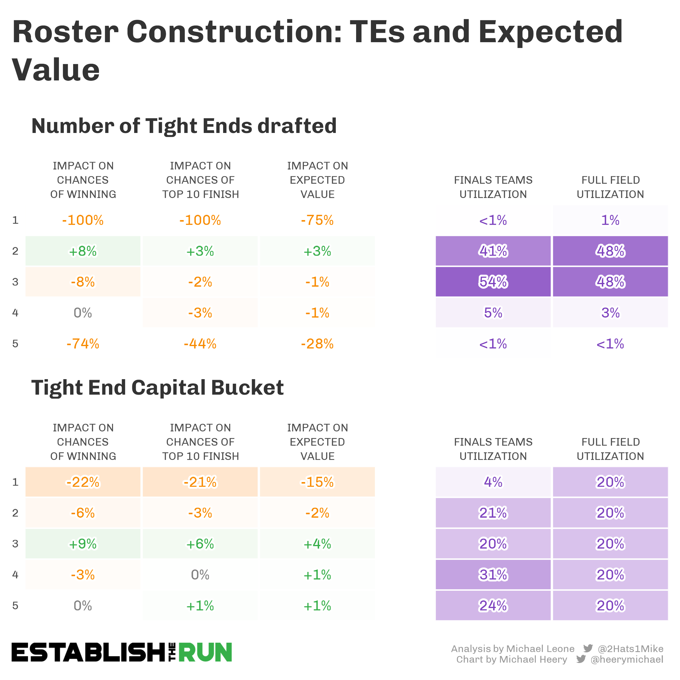
Key Notes:
- Aside from having a positive expectation in finals participation rate, 4-TE teams held their own in terms of finals EV, posting pretty neutral EV and Win % averages.
- There were only three combined TE teams that rostered 1 or 5 TEs, but all 3 of these extreme builds had a very low finals EV.
- Following suit with the finals participation rates, teams in TE capital buckets 1-2 also were -EV in Week 17 specifically.
I want to repeat for the umpteenth time that it’s good to understand last year’s data and dissect it; it’s not good to assume it’s predictive. I don’t think the data last year suggesting late TE is good and elite TE is bad is likely to continue this season. 2023 was an outlier year in terms of poor production from the earliest drafted TEs and a couple of rare breakout TE performances from late round TEs (LaPorta, McBride). And likewise, 2 TE teams underperformed relative to 3 TE teams not necessarily because that structure was worse, but because many of the 2-TE teams were elite TE teams while the 3-TE teams were less likely to be elite TE teams and more likely to have rostered LaPorta or McBride.
Many of the sharpest BBM drafters that I know are heavily into Elite TE this season. I still think 3-4 late TEs can work if the value doesn’t support an early TE selection, but quite often the value does support it. In other words, I’m not forcing an Elite TE build currently, but if you’re drafting off of our ranks and catching falling ADP values when they’re there, you should be getting a TE in the first 6 rounds at a higher rate than the field.
I hope you found this article helpful in terms of getting your mind thinking about what it takes to compete in Week 17 without sacrificing your ability to get there. While this analysis is based off a very small sample (one week for one year of data), it hopefully helps to capture some of the nuance that is left out of my Best Ball Manifesto where I estimate finals win rates using threshold scoring (which ignores pod variance and the consecutive nature of the playoff stages).