Best Ball Mania Manifesto: A Guide To Winning Big On Underdog Fantasy

To get access to all our continuously updating Best Ball Rankings + Content, head here. It’s just $39.99/year.

 

Best Ball Mania III was the most popular season-long fantasy tournament of all time, paying out an incredible $2 million to first place. This series is a deep dive into the optimal strategies we believe make sense in a tournament with this structure.

The series is broken into four parts, which roughly cover: stacking, ADP value and what types of drafts you should join, roster construction, and then putting everything together to calculate expected value for teams in this tournament.

Each part will be added to the bottom of this article when it is released, creating one large manifesto. We’ll include jump links so you can directly navigate to the part you’re interested in.

 

Best Ball Mania Manifesto
Introduction
Part 1 – Stacking
Part 2 – ADP Value
Part 3 – Roster Construction
Part 4 – Grading Drafts

 

Introduction

The introduction takes a look at the structure of the Best Ball Mania tournaments and some of the conflicts that arise when trying to optimally build teams for the contest. The short and sweet intro is:

• Best Ball Mania’s payout structure puts all of the leverage in the playoff weeks, particularly the final week.
• The playoff structure can lend itself to randomness because it is designed as three separate but consecutive top-heavy tournaments.
• We want to position ourselves as strongly as possible to take advantage of the unique playoff structure while also getting as many teams through to the playoffs in the first place.
• In order to do so, we need a better understanding of the levers we can pull in a draft (stacking, value, roster construction) and how those impact regular-season advance rates and estimated playoff win rates.
• Finally, we need to marry regular-season advance rates and estimated playoff win rates and how each impacts the overall Expected Value of a team so that we know what to prioritize when drafting.
• Put most succinctly: What this manifesto sets out to do is to figure out what drives success in the best ball playoffs so that we can more strategically find the balance between high regular-season advance rates and optimally-built playoff teams.

 

Playoffs Are Where The Money Is

In past years, we’ve analyzed Underdog Best Ball Mania data to determine which strategies and roster constructions give teams the best chance to advance out of the regular season (finish top two in a 12-team league in Weeks 1-14). We’ve focused on this data for a few reasons:

 

1. League advance rate is a bit more controllable than success in the playoffs.
2. This information is useful for all best ball leagues on Underdog, not just Best Ball Mania.
3. Most simply, this data has been the easiest to analyze because of its availability and sample size.

 

However, as much quality analysis throughout the industry showed last year, including Peter Overzet’s Week 17 Is All That Matters video, the most important weeks in Best Ball Mania are specifically the playoff weeks. The expected value of a team increases exponentially as you move through each round from the regular season to the quarterfinals, to the semifinals, and finally to the Week 17 finals.

I stumbled across this Tweet from Ben Dominguez a few weeks ago, who has been providing great data science visuals:

 

My immediate response was: “We need to think of upside through the lens of playoff upside, not total points across the season.”

The leverage in the playoff weeks grows as the top-heavy prize pool grows. Last year, Pat Kerrane took down a $2 million grand prize, finishing in first place out of 470 teams that made the finals. The team in 470th? It took down $1,000.

There’s a lot of chaos in these weeks, much of which is out of our hands, and that does mean we want to focus on advancing as many teams to the playoff stages as possible to increase our odds of getting lucky.

However, given the importance of the playoff weeks and as rich of a dataset as we’ve ever had (over 75,000 playoff teams in last year’s Best Ball Mania contest), I wanted to dig in and see if we can cut through the randomness of the playoff weeks and parse out if any roster construction or macro strategies give people a better chance of succeeding once they get to the playoff stage. But a little more context first…

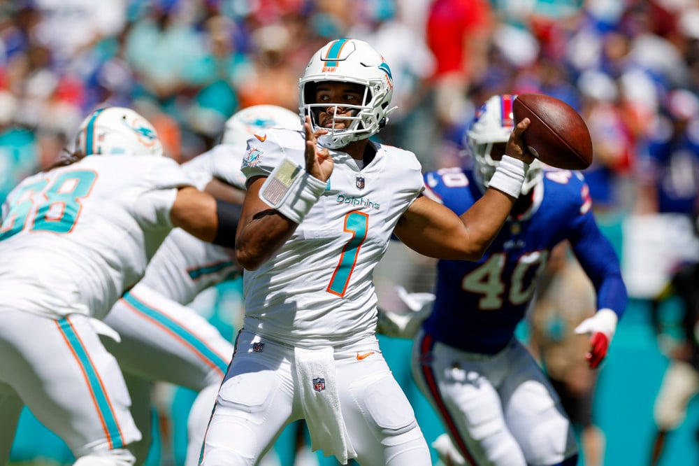
The Winner of BBM3 and a cool $2 million grand prize, Kerrane, was inspired by the above linked Week 17 Is All That Matters video, and it showed on his winning team:

 

Pat had three QB stacks and two Week 17 game stacks:

• Tom Brady–Chris Godwin–D.J. Moore
• Tua Tagovailoa–Jaylen Waddle–Mike Gesicki–Raheem Mostert–Jakobi Meyers–Tyquan Thornton
• Daniel Jones–Wan’Dale Robinson–Saquon Barkley

 

The results are interesting. Game stack 1 paid off hugely, as Tom Brady was the highest-scoring QB on the slate, and the heavy correlation in that game resulted in strong WR scores from Chris Godwin and D.J. Moore. It’s worth noting that Mike Evans had the highest-scoring WR game of the entire season as Brady’s primary recipient in this game.

The other stacks had more mixed results in terms of correlation. Daniel Jones had a massive score, as only Brady scored higher. It’s a bit ironic that a 3-QB strategy, where you’re theoretically accepting less individual upside on a weekly basis, netted Pat the top two scoring QBs on the week. However, Jones hit his upside primarily on the ground, which resulted in an unusable score from Saquon Barkley. Stacked WR Wan’Dale Robinson was injured.

The other big game stack of MIA-NE hit but in a somewhat uncorrelated way. Tua was injured, and all of the MIA pass catchers failed to produce usable scores. However, Raheem Mostert, Jakobi Meyers, and Tyquan Thornton all posted usable scores. It’s tough to tell how correlated this all was, as it was a predictably low-ish scoring game (23-21 with a D/ST TD) with around an average amount of plays run, but Pat’s players ended up scoring four of the five offensive TDs in the game. Mostert did most of his damage via receiving work.

Pat’s team spells out the conundrum in analyzing strategies for Best Ball Mania and any format where the playoff weeks are so important and so top-heavy. Two of the three stacks didn’t really see a benefit from correlation despite having strong Week 17 performances, but the stack that did benefit was absolutely critical to Pat’s success.

On the other side of the coin, some elements that had nothing to do with stacking and more to do with randomness were also critical to Pat’s success. A low-owned Austin Ekeler went off while high-owned Justin Jefferson and, ironically, Saquon Barkley failed. The heavily correlated BUF-CIN game among finalists was canceled. Pat’s team was extremely healthy as well. 15/18 of his players recorded a non-zero score in Week 17, something we will see massively boosted his odds when the second part of this manifesto is released below. His injuries were his second-drafted QB of three, a late-round RB, and a late-round WR.

There was also some clear intention in Pat’s strategy at work beyond stacking, such as a 3-QB structure and banking on RBs he felt were worth a very early pick:

 

Additionally, Pat’s team was in the Top 90th-100th percentile bucket in terms of ADP Draft Capital (more on this in Part 2) and Top 80th-90th percentile in a more simply derived ADP Value metric (actual pick number — final ADP for all of his players).

 

In essence, there are two extreme mindsets when it comes to drafting a Best Ball Mania team.

• The playoffs are random, so focus all of your energy on drafting teams with the highest possible regular-season advance rate and hope to sun run.
• The playoffs contain all of the leverage given the payout structure, so focus all of your energy on drafting teams with high weekly upside that are optimized for the playoff weeks. You may get fewer teams through to the playoff round, but those that do get through are more likely to sun run.

 

The truth, as always, lies somewhere in the middle, and I don’t think anyone participating in BBM would argue otherwise. People who are drafting to optimize their playoff stacks aren’t ignoring draft day value and roster construction techniques that promote regular-season advance rates. People who draft trying to optimize their regular-season advance rate aren’t ignoring their pass-catcher stacking potential and Week 17 opponents. What this manifesto sets out to do is to figure out what drives success in the playoffs so that we can more strategically find the balance between high regular-season advance rates and optimally-built playoff teams.

 

Methodology

This article contains two types of analysis.

The first type is straightforward — analyzing all of the Best Ball Mania teams through the lens of advance rate (making it out of the regular-season stage and into the quarterfinals).

The second type of analysis is a bit more complex, as we attempt to tease out the weekly upside of those teams that made the quarterfinals.

As I noted above, 75,200 playoff teams gives us a pretty big sample to work with. However, there is just one quarterfinals week, one semifinals week, and one finals week. So only using actual playoff results fails to give us much of a signal, since the outlier individual fantasy performances of players in a single week are going to shape the results to a high degree, no matter how large the sample of teams is.

To give us a better sample, I decided to take all of the playoff teams in last year’s Best Ball Mania and test their ability to achieve the requisite weekly playoff upside by looking at their percentile outcomes amongst each other for all 17 weeks.

For each team and each week, I determined if their weekly score was high enough to be credited with an “estimated win”. To get credited with an “estimated win” in the quarterfinals, you needed a top 1/10 score; for the semifinals, a top 1/16 score, and for the finals, a top 1/470 score. Of course, for the finals, any outcome in the top five is quite strong. I did not simulate consecutive weeks (quarters – semis – finals), as I’m purely looking to see if the weekly upside matches what is needed to win a quarters, semis, or finals.

This now expands our sample quite a bit. Even for testing which teams have enough upside to win in the finals, we have a sample of 160 teams (out of 75,200) that finished with a top 1/470 score for each of the 17 weeks (7,140 teams), which is pretty good.

Now, this isn’t a perfect analysis because some of the weeks before the playoffs aren’t perfectly reflective of what we’ll see in the playoffs. At the beginning of the season, there has been less time for injuries and younger player breakouts to occur. In the middle of the season, there are bye weeks. I also didn’t account for the randomness of playoff groupings, which might reduce the observed impact of any strategy or technique. Ultimately, though, the size of the sample makes this analysis way more valuable than simply analyzing the playoff weeks by themselves.

Any backward-looking analysis also has its limits. Each year, the player pool changes, the ADPs change, and the strategies drafters use change, which means what has or has not worked in the past isn’t necessarily reflective of what will or will not work this season. It’s important to think critically when digesting the following results.

 

Part 1: Stacking

Part 1 of the Best Ball Mania Manifesto concentrates on the impact of stacking. Here’s a high-level summary if you are mostly interested in just the results:

• We want to find the balance between optimizing teams for the playoff stretch in big best ball tournaments while also being realistic about where we have the most control.
• Stacking has become table stakes. Roughly 10.5/12 people in every league are stacking to some degree, and it creates a small edge in advancing out of the regular season.
• Week 17 game stacking was a popular topic last season, and the data shows that your ability to win a 470-person field can increase by ~50% by game stacking.
• Game stacking also helps you win 10-team (reflective of quarterfinals) and 16-team (reflective of semifinals) pods, but the increase in performance isn’t nearly as large as it is in the finals.
• Two QBs are better than three QBs, but you should try to stack each QB as much as possible.
• In the regular season, having 3-5 of your skill players stacked with your QB was optimal. So, you don’t need a huge team stack; 1-3 stacked players per QB is optimal.
• In Week 17, ideally, you have between 6-9 total game-stacked players, where a player is considered “game-stacked” if they are on the same team as your QB or any opposing skill player.
• If you mass-enter 150 teams into Best Ball Mania, the EV of 30 advancing teams that are structured near optimally in game stacking is roughly the same as advancing 35 “random” teams.

 

Regular Season

Starting in the regular season, we see that stacking helps advance rates. There are a few reasons for this, but chief among them is the simplest: If an offense performs well throughout a season, everyone benefits.

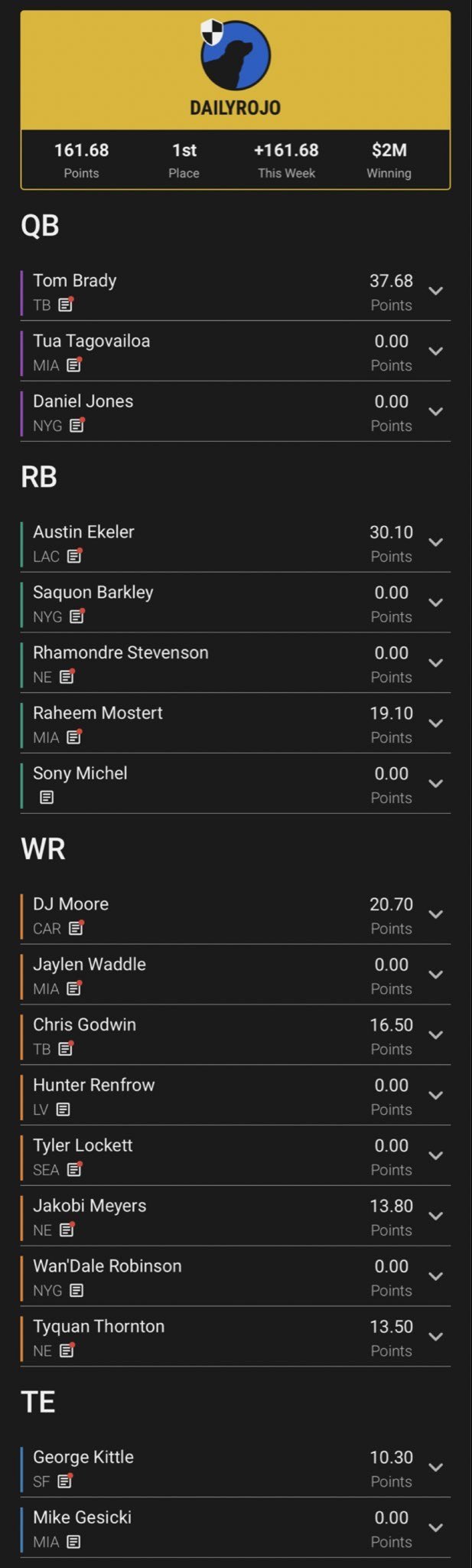
General notes on regular-season stacking:

• No QBs stacked is by far the worst advance rate.
• Two is better than three, but there’s a bias here in that two QBs, in general, is better than three QBs. If you have three QBs, it’s best to stack all three of them.

 

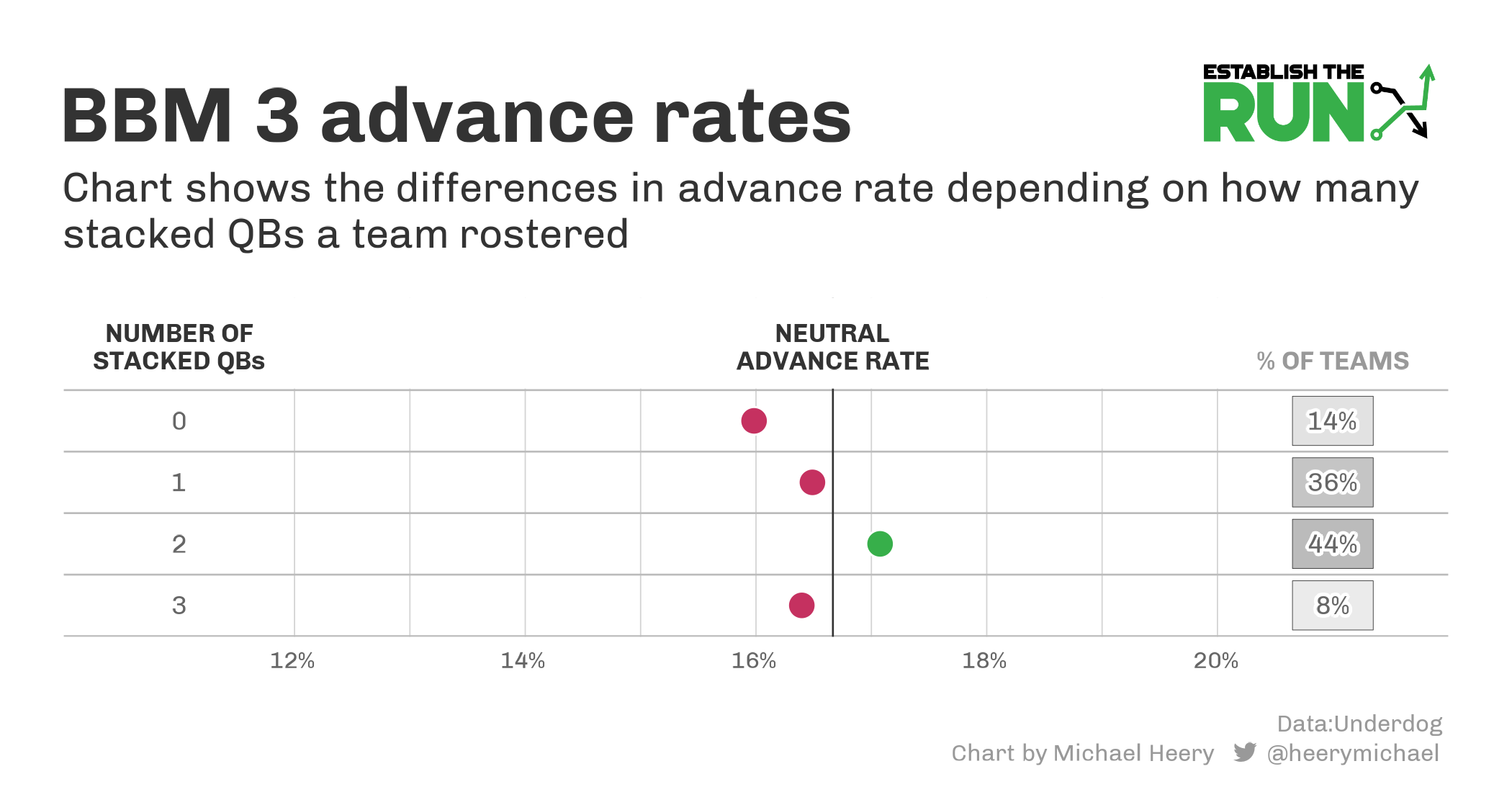
Let’s look at this spliced up a bit more, combining the number of QBs on the roster with the number of QBs stacked.

Notes:

• You should never draft anything but two or three QBs.
• When drafting two or three QBs, the more of those that are stacked, the better.

 

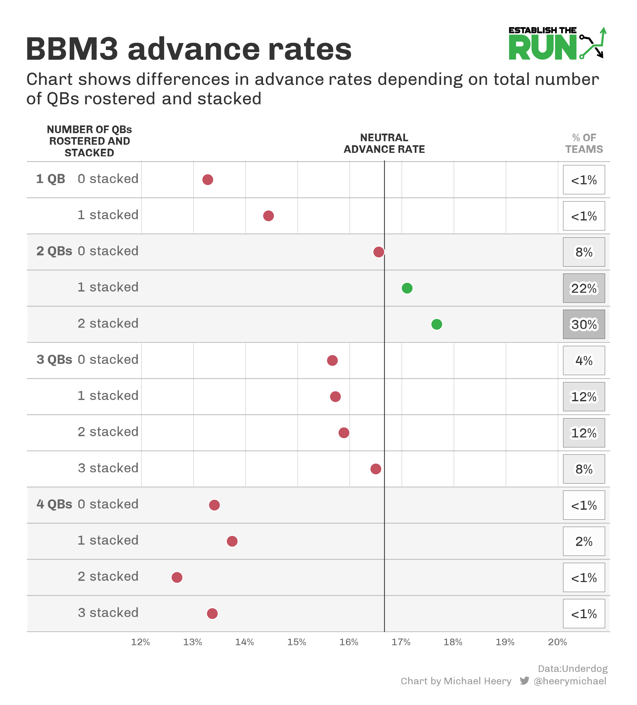
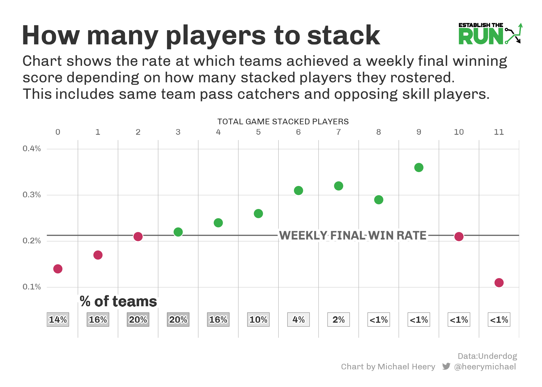
You should try to stack, and it will be more clear when we look at the playoff data. Sticking to the regular season for one more visual, though, how many of the skill players we draft should be stacked with our QBs?

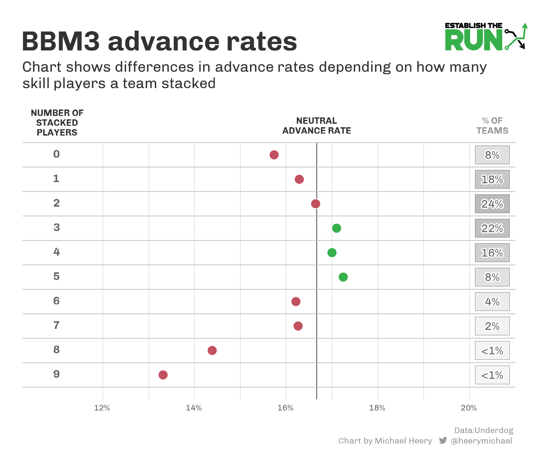
Notes:

• Keep in mind this is all skill players stacked (includes RBs, playoff analysis will exclude same-team RBs).
• Having only one or fewer skill players stacked is bad, which is obvious because you’d need at least two to stack two QBs.
• There’s not a huge difference in advance rates once you’re stacking at least two skill players but not more than seven. Between three and five seems best, which is roughly 20-33% of your non-QB roster spots (a little less if only rostering two QBs).

 

You should be trying to stack as many QBs as you have rostered if possible in the regular season, but these don’t have to be huge stacks. With the total number of stacked skill players being in that 3-5 range, that means you’re likely only stacking 1-3 total players with each individual QB.

What’s also clear is how prevalent stacking has become. Only 13.7% of contestants aren’t stacking at all; that’s a little bit more than 1.5 teams per league. Some form of stacking is table stakes in the regular season.

 

Playoffs

We can slightly improve our regular-season advance rates by stacking, but the proceeding playoff analysis shows that stacking helps achieve the weekly upside needed to win the three different playoff stages, particularly the finals, where the majority of the money is handed out.

Let’s look at the estimated win rates for the estimated quarterfinals (a top 1/10 score in a given week), semifinals (top 1/16), and finals (top 1/470) among the 75,200 teams that made the playoffs, essentially treating each team as 17 different teams for the 17 different weeks. Please note that the estimated win rates referenced for the playoff weeks are based on *if* a team makes it to that week. So, when you see a finals estimated win rate of 0.25% in a chart, that means that team has a 0.25% chance of winning a 470-team field size in a single week. It does not mean they have a 0.25% chance of winning Best Ball Mania III. The EV calculations explained later on take into account the odds of winning a finals week with the odds of getting there in the first place.

 

For the following stacking data:

• RBs are not included for any of the team stacking data.
• For game stacking, opposing RBs, WRs, and TEs are included.
• A game stack must include a team stack (QB with at least one same-team pass catcher) and a bring-back (QB with at least one skill player from the opposing team).

 

Now here’s a look at all the estimated win rates based on team stacking and game stacking across the three playoff stages:

If that table is too dense, here’s a simpler look:

Notes:

• Stacking is powerful in the playoffs, especially as group sizes expand.
• It appears having three QBs stacked, particularly game stacked, is better than having just two QBs, despite two QBs performing better than three QBs in isolation (this will be disproven a little later on).

 

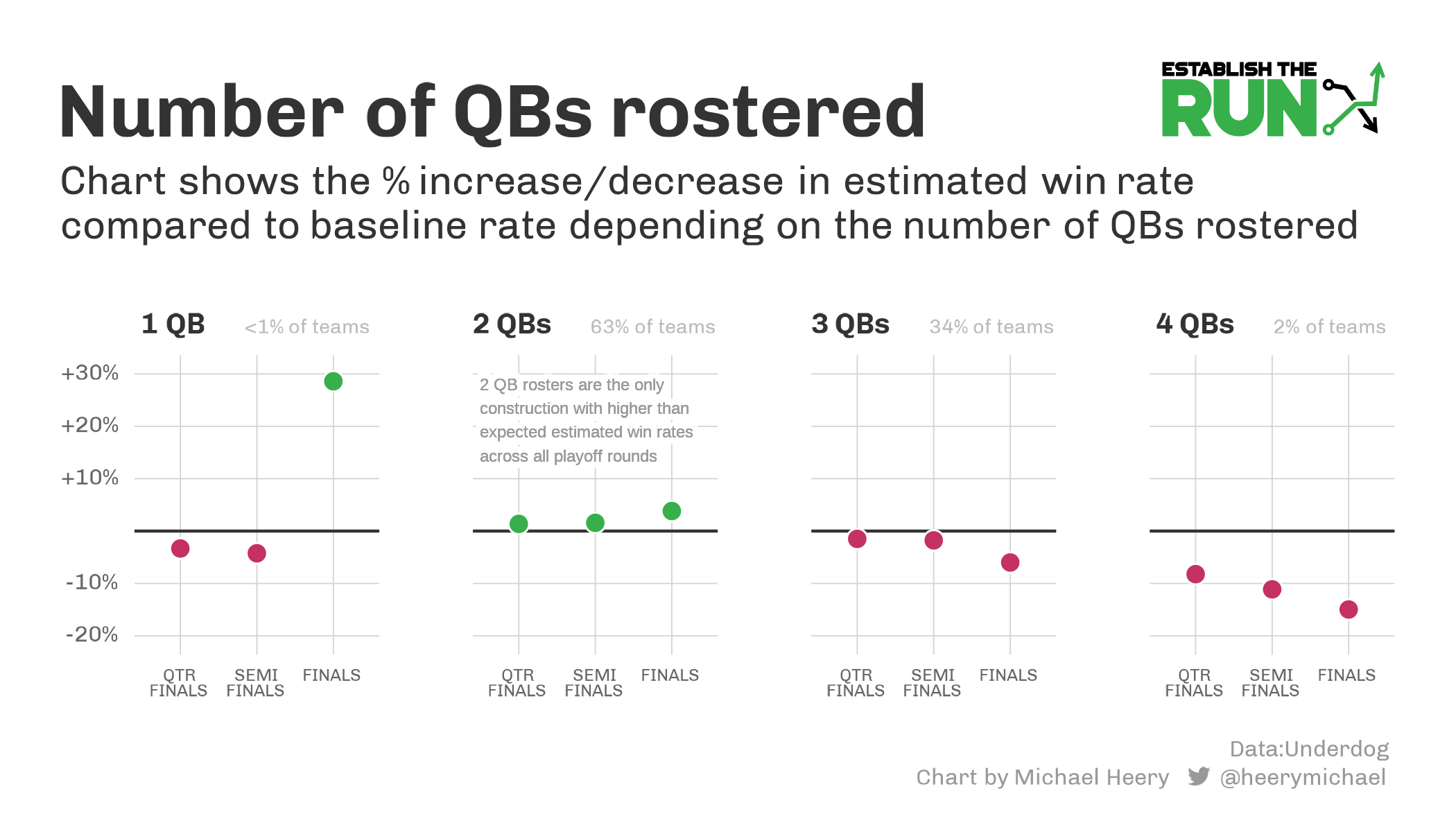
As an aside, the number of QBs rostered visual showcases an example of why we need to look at all of this data in conjunction. Looking at the above visual in isolation could lead one to believe that playing a 1-QB team is +EV given its strong finals win rate.

 

However, 1-QB teams:

• Have a poor regular-season advance rate
• Are unable by definition to have multiple game stacks, which buoy the 2- and 3-QB teams’ finals win rate potentially even higher than 1-QB playoff teams

 

In light of trying to put everything together, let’s see if we can back into a rough Expected Value (EV) of a playoff team based on structure.

Playoff EV = (Odds of losing in quarters*average quarters loser payout) + (Odds of losing in semis*average semis loser payout) + (Odds of losing in finals*average finals payout) + (Odds of winning finals*finals grand prize payout)

Note for this thought exercise specifically, we’re looking at the EV *after* a team has advanced out of the regular season, so regular-season advance rates are ignored.

This is imperfect, as payouts vary when you lose in a round based on where you finish. It’s particularly flawed for the finals where coming in second is worth $1,000,000, but coming in 470th is worth $1,000. Still, this is a quick and easy way to visualize how changing advance and win rates truly affect what we care about — the money we’re likely to win.

 

The average EV of a quarterfinals team is as follows (some small rounding errors may exist):

90% chance of losing in quarters * $37.22 average payout = $33.50

9.4% chance of losing in semis * $137.63 average payout = $12.90

0.624% chance of losing in finals * $9,619 average payout = $60.00

0.0013% chance of winning finals * $2,000,000 grand prize = $26.60

TOTAL EV = $33.50 + $12.90 + $60.00 + $26.60 = $133.00

 

For a reference point, let’s once again take a look at the visual of playoff teams based on the number of QBs on the roster, this time with an EV calculation:

Interestingly, you see that 1-QB teams have a lower EV than 2-QB teams despite a better finals estimated win rate because the odds of a 1-QB team even making it to the finals in the first place is lower (and this is assuming the 1-QB team makes it to the playoff stage in the first place). In fact, a 2-QB structure was the only structure that had an estimated win rate above expectation across all of the playoff stages.

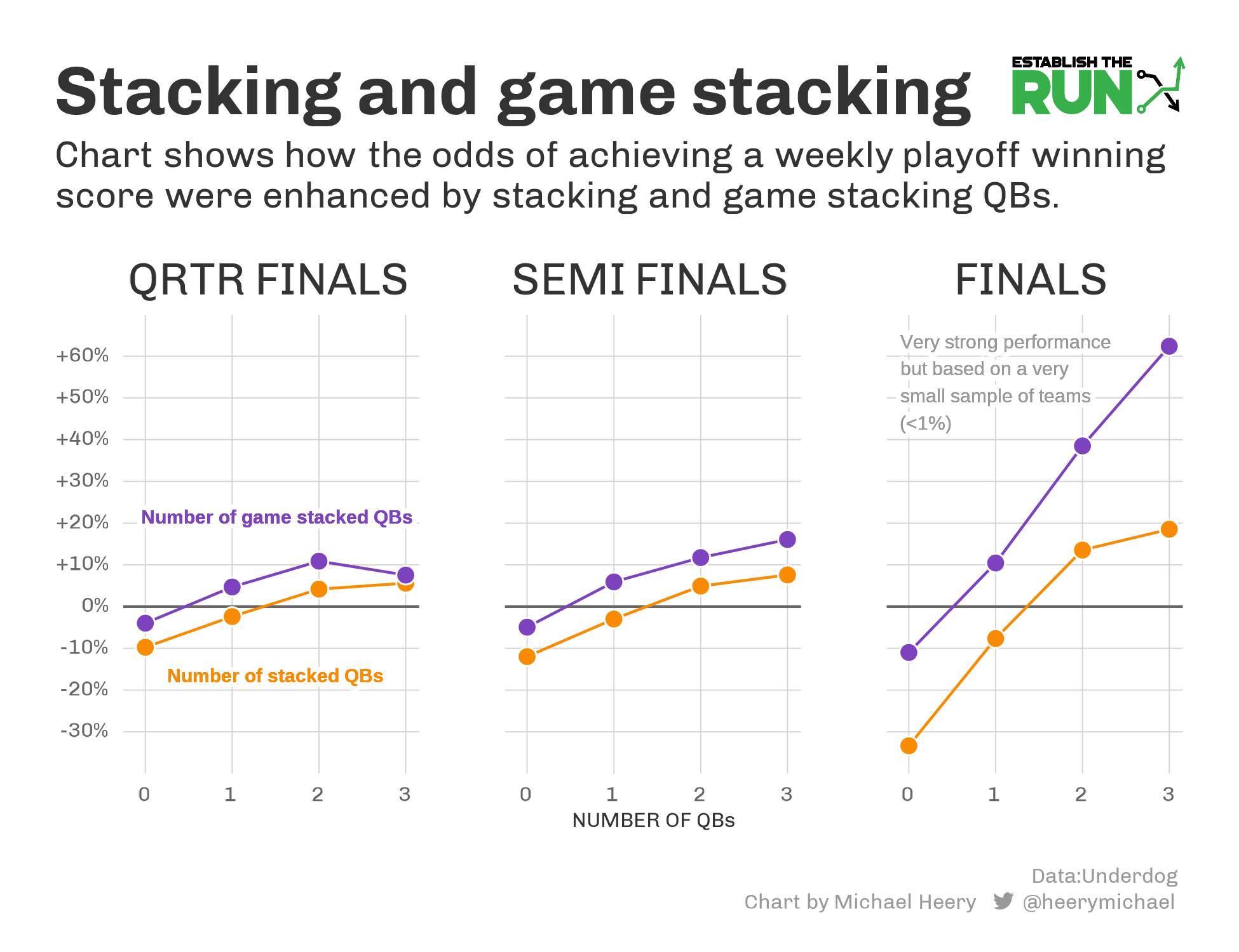
Bringing it back to correlation with your QBs, it’s good to know that game stacks improve your odds of winning across all of the playoff stages. However, it’s most important to game stack in Week 17 (both the highest-leverage week and has the largest impact on improving your odds of hitting the necessary upside threshold), and it’s nearly impossible to plan multiple game stacks in Week 17 while also planning stacks in Weeks 15 and 16 (though it’s worth keeping in mind).

So, to get a better sense of the EV improvement by having Week 17 game stacks, we can use the semis and quarters estimated win rates from stacked teams. For example, if a team has three game stacks for Week 17, it necessitates they at least have three team stacks for the quarters and semis since you can’t have a game stack without the team stack. For a team with two Week 17 game stacks, we’ll use the weighted odds of that team having a 2- or 3-QB team stack and so on.

The EV of teams with zero and one QB game stacked is probably lower, as I’m likely overstating the odds they had 2+ QBs team stacked.

To put this into perspective, I’m on record as saying I’d rather have 35 random teams advance out of the regular season than 30 playoff-optimized teams.

I won’t cherrypick the absolute nuts data from above, since it’s not necessarily realistic to be able to stack all of your QBs up in a Week 17 game stack fashion. It does seem realistic to design a team that has roughly a $150-160 EV entering the playoffs.

30 teams at a $150-160 EV = $4,500 to $4,800

35 teams at a $133 EV (EV of a random team) = $4,655

This data might look contrived, but it earnestly came about and ended up in a spot where 30 “optimally” stacked playoff teams is essentially breakeven with 35 random teams.

 

As a side note, I was surprised that the impact of game stacking was so powerful, especially since team stacking in isolation was solid but not surprisingly powerful. I had two concerns that I thought might impact the data:

• Is including bye weeks in the analysis distorting the data?
• Is including early-season weeks distorting the data?

 

The short answer: The data did not change in any meaningful way after accounting for either bye weeks or early-season weeks.

Like with the regular-season data, it’s clear that stacking (and Week 17 game stacking in this case) is important to accomplish with as many QBs on your roster as possible, but we want to try and figure out how big these stacks should be.

Putting it all together:

• Have multiple Week 17 game stacks
• Overall 6-9 combined same-team pass catchers and opposing skill players in Week 17
• 2-3 pass catchers with QB1
• 2-4 pass catchers with QB2
• 2-4 pass catchers with QB3

 

In Part 2 of this series, I’ll try to better answer the question of “How much value in a draft should I give up to complete a stack?” Clearly, stacking is important in the playoffs, but we still need to know when we’re faced with a decision in a draft where we should go when considering all information, most notably prioritizing advance rate or playoff optimization. ADP value has a higher correlation to regular-season advance rate, while stacking structure has a higher correlation to estimated playoff win rates.

We can look at whether or not you should draft two or three QBs as an example of how we can answer this type of question. We know that drafting two QBs has a better advance rate and playoff win rates in general. However, if we’re able to game stack three QBs for Week 17 (thus by definition having three QBs team stacked for all prior weeks as well), the playoff win rates start to balloon. So what should we do?

Let’s extend the EV calc I worked on above to include the regular-season advance rate data.

What we see here is that it’s critical to stack your QBs if drafting three of them to make up for the better structural edge 2-QB teams have, stacking aside. In the above data, whenever the number of team stacks and game stacks were the same, the 2-QB side had a higher EV. For example, if you had two team stacks and one game stack, rostering two QBs netted an EV of $27.38 compared to just $21.60 for 3-QB teams.

Putting it all together, we see that the critical piece is trying to stack the maximum number of QBs possible, whether you roster two or three, and in most cases, doing so with two QBs is better than with three QBs. So while a previous visual looked really kind to game stacking three QBs, which you can only do if you roster three, we actually see that rostering two QBs but being able to game stack them both is more powerful ($31.28 EV to $29.50 EV).

 

If you’re curious about how sensitive this data is in terms of regular-season advance rate, here are some thresholds:

For a 3-QB team that is game stacked across the board to become neutral EV ($22.20), the advance rate would have to drop from 16.5% to 12.4% (assuming the playoff stage win rates hold). We’ll look at this in more detail in Part 2, but that’s roughly akin to losing 72 spots of ADP value across your entire team. Of course, the decision is rarely black and white, one thing or another, but it’s good to have a frame of reference.

Conversely, for a 2-QB team that is not stacked at all to reach neutral EV, their advance rate would have to climb from 16.6% to 20.6%, roughly akin to gaining 72 spots of ADP value this time.

ADP Value is defined as overall draft pick number minus final ADP. So a player you drafted 13th overall who finished the draft season with an ADP of 10 would be an ADP Value of 3. Again, we’ll have more on this in Part 2.

 

Caveats

With the simplicity by which this analysis was done (looking at Top X% weekly scores), there are some nuances of the playoff format not covered.

Most notably, the figures above are purely descriptive and not predictive. We shouldn’t treat them as gospel, especially in instances like the last example where we’re chopping up the data in a few different ways, making the results more prone to noise.

The randomness of the pods in the quarters and semis would likely slightly dampen the effect of stacking (or any edge case because more variance is introduced). Along these same lines, I do wonder if a 3-QB team may have a bigger edge if you were to simulate the playoff weeks consecutively (three weeks in a row), rather than looking at them all in isolation as I did.

While the pods themselves are random, the teams that advance to the semis and then to the finals are correlated in terms of the players on the roster. As a result, game-stacking efficacy may be slightly reduced because its uniqueness is likely reduced. The latter point is likely to have a more meaningful impact than the former, but this data is still a win for prioritizing Week 17 game stacking given its ability to increase the odds of putting up a Top-1-out-of-470 weekly score. 

Finally, keep in mind this is based on all 17 weeks of data. So while people were consciously building out Week 17 game stacks, most of the data set I am working with is from Weeks 1-16. The game stacks on the opponent side then were the result of random alignment on those weeks. These were stacked teams that coincidentally also had an opponent of their stacked team for that particular week, whether it was Week 3 or 10. Those game stacks of happenstance are likely to be a bit more value-conscious than the intentional Week 17 game stacks and composed of players taken earlier in the draft (as opposed to filling out late rounds simply based on Week 17 correlation). I don’t think this would move the needle much, but it’s worth pointing out, especially since we’re likely to see people go out of their way to stack even more this season, which could bring down the true EV of these teams in the playoffs if they do a poor job in doing so.

 

Part 2: ADP Value and ADP Draft Capital

Part 2 of the Best Ball Mania Manifesto concentrates on the impact of ADP Value, live players, and which drafts to join. Here’s a high-level summary if you are mostly interested in just the results:

• Achieving closing line ADP Value only has a small impact on estimated playoff win rates.
• However, it has a meaningful impact on regular-season advance rates.
• This is important because regular-season advance rates have a significant impact on the estimated Expected Value of a team.
• As a general rule of thumb, every 1-percentage-point increase in estimated regular-season advance rate is as beneficial as a 4-percentage-point increase in estimated finals win rate.
• Estimated playoff win rates are heavily influenced by the number of live players on your roster.
• Drafting in July and August provides a nice balance between increasing your odds of achieving strong closing line ADP Value and having a higher number of live players on teams that advance out of the regular season.
• Slow drafts make it tougher to achieve strong closing line ADP Value, but the impact is pretty small.

 

We saw in Part 1 that varying levels of stacking can slightly improve your advance rate and greatly improve your odds of winning the playoff stages, particularly the finals.

Can drafting teams based on value replicate similar improvements in Expected Value? If that’s the case, draft day decisions can still remain muddy in gray areas of the draft when deciding between taking a stack partner and taking a much better value. If not, draft day decisions become clearer, as making the correct stacks would remain our top priority.

I ranked all teams in Best Ball Mania 3 based on ADP Value. ADP Value is calculated by taking where a player was drafted minus their final ADP in the contest. So, if you drafted Amon-Ra St. Brown 70th overall in June, and his ADP in the contest closed at 46, your ADP value for that pick is 24 (70 minus 46). A team’s total ADP value is the ADP value of all 18 picks added together.

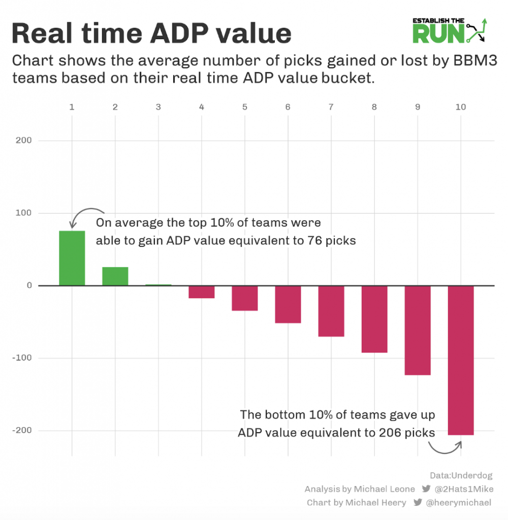
I then bucketed each team’s ADP Value into percentiles of 10. ADP Value Bucket 1 means you were in the 90th-100th percentile for ADP Value (i.e., you had the best ADP Value). ADP Value Bucket 10 means you were in the 0-10th percentile (you had the worst ADP Value). Here’s the average ADP Value of those buckets:

 

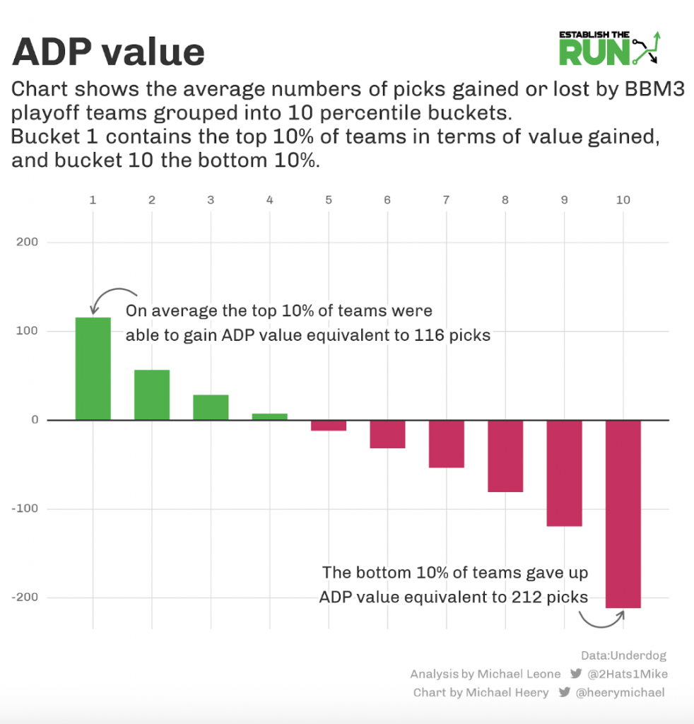
I was surprised at how wide-ranging these values were given a relatively large bucket size. Even between buckets in the middle, we see large gaps. Teams in Bucket 4 (60th-70th percentile) had on average 39 more spots of ADP Value than teams just two buckets down in Bucket 6 (40th-50th percentile).

And obviously, on the ends, we see that 10% of teams were able to get massive ADP Value in their contests, well above any other bucket, while 10% of teams were on the opposite end of the spectrum.

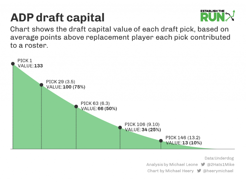
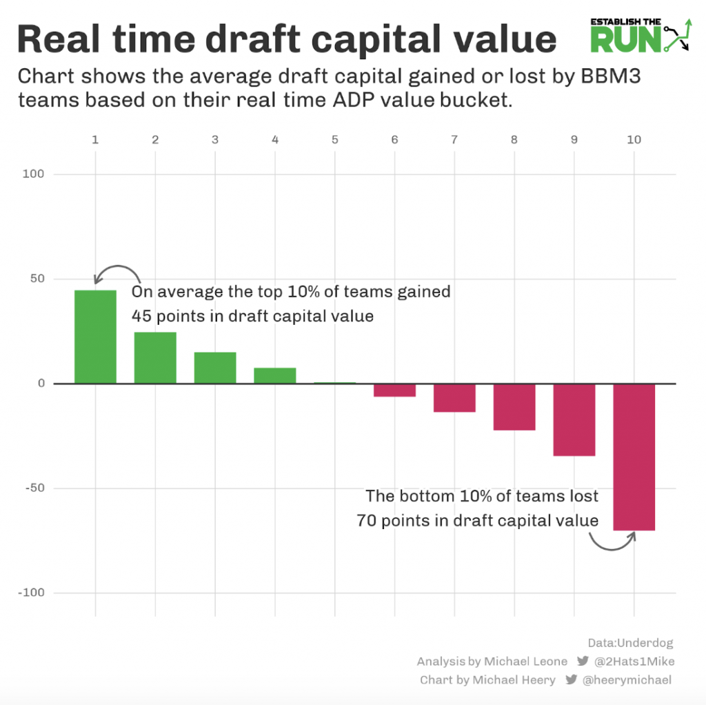
In addition to looking at ADP Value, I trained a simple model to give each draft pick a “draft capital” number by looking at the average points above replacement player each pick contributed to a roster based on where they were drafted.

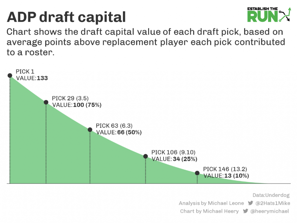
The above visual gives you an idea of how draft capital scales, allowing us to account for the non-linear nature of draft value. Picks earlier in the draft are worth more draft capital than picks later in the draft, so giving up ADP Value in the second round is a bigger deal than giving up ADP Value in the final round.

Each team in BBM has around 786 points of draft capital to start, varying slightly based on draft slot. We can see how much draft capital value they earned by using a player’s final ADP to calculate draft capital rather than the pick number. For example, if you drafted a player at pick 63, that would be 63 points of draft capital. But if their final ADP was 29, their ADP Draft Capital would be higher (100).

If you’re interested in the exact draft capital by pick, you can find it in this Google Sheet.

Similar to ADP Value, I split up ADP Draft Capital into 10 buckets:

 

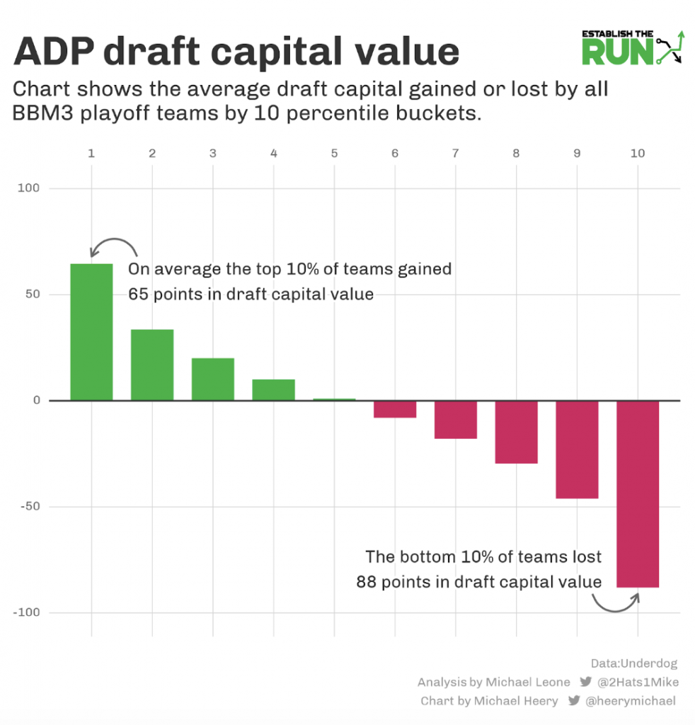
As you’ll see, ADP Draft Capital didn’t add any signal ADP Value didn’t pick up on when we do a cohort analysis of regular-season advance rates and estimated playoff win rates, but the concept of pick draft capital will be important in Part 3 as a more nuanced way to look at roster construction.

 

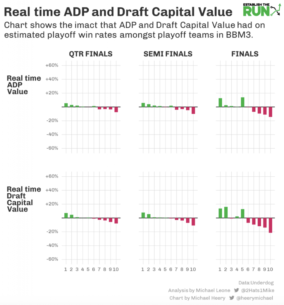
Estimated Playoff Win Rates

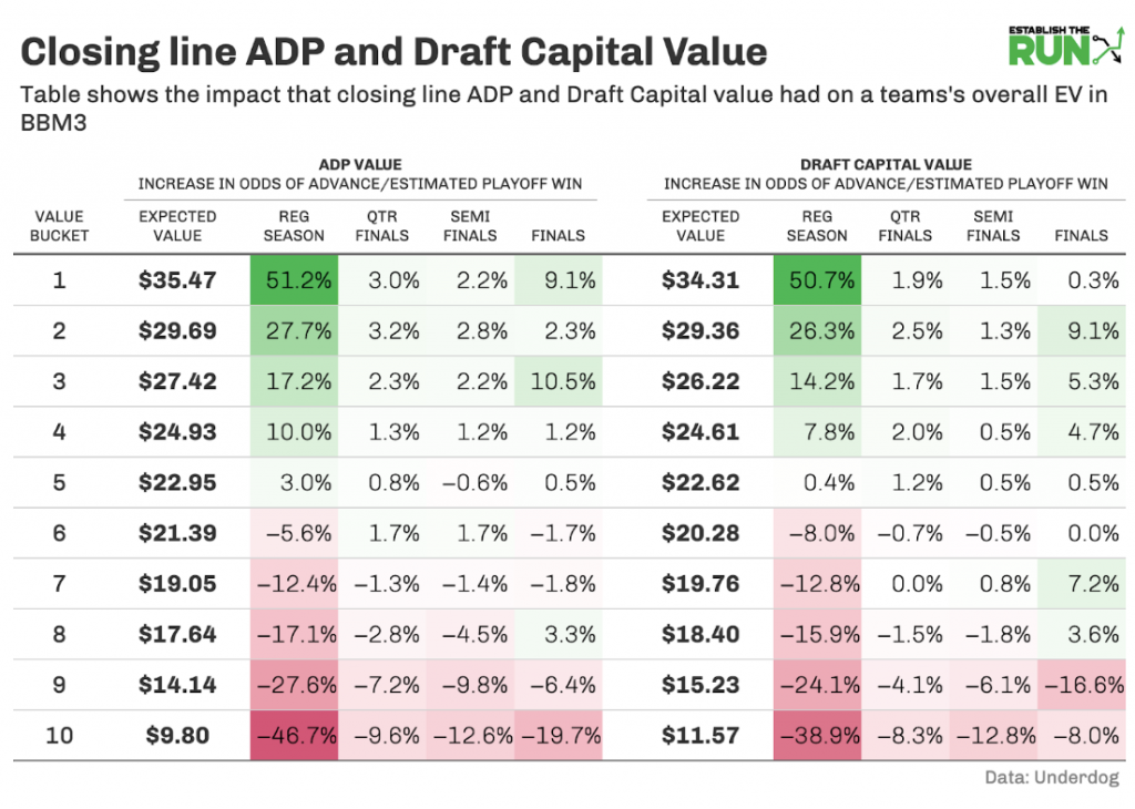
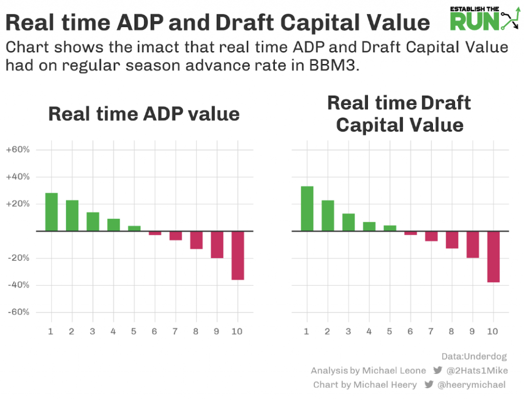
So, we saw in Part 1 that stacking had an important effect on estimated playoff win rates. Let’s see if that holds true for ADP Value and ADP Draft Capital:

 

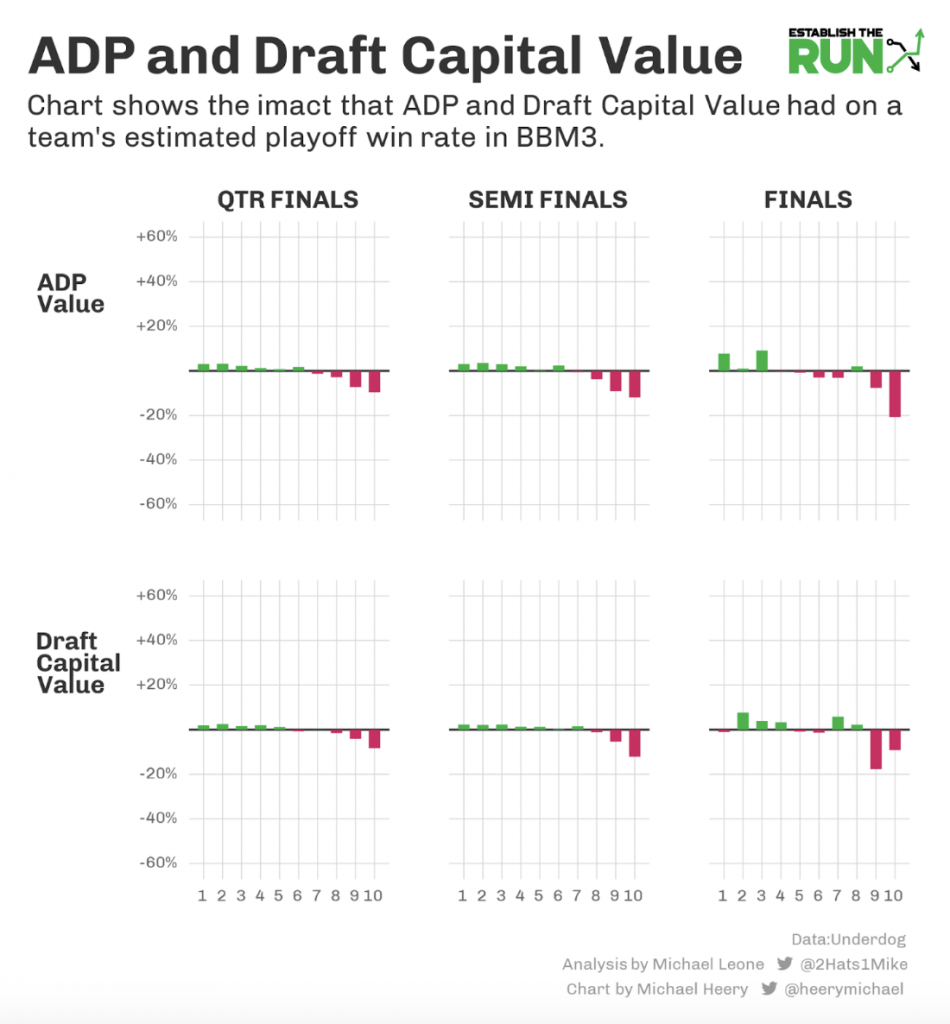
Notes:

• The trend is positive, but the magnitude is small.
• It’s good to be in the top 3-4 buckets, and really bad to be in the bottom two buckets, but there’s not a ton of change from bucket to bucket.

 

At this point, stacking over value looks obvious as far as priorities go. But what we’ll see is that the EV of a team can be altered heavily by advance rate expectation, even if playoff estimated win rates aren’t changed meaningfully.

Here are the regular-season advance rates based on ADP Value and ADP Capital:

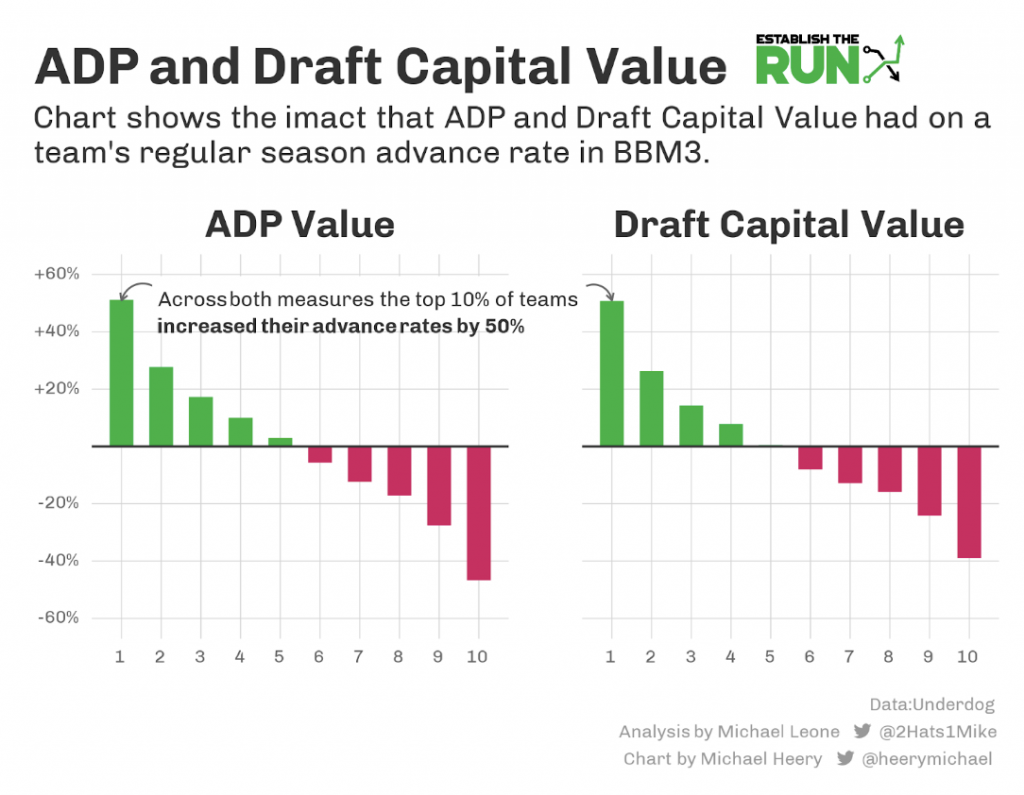
The trend is extremely consistent, and the magnitude is higher than I expected.

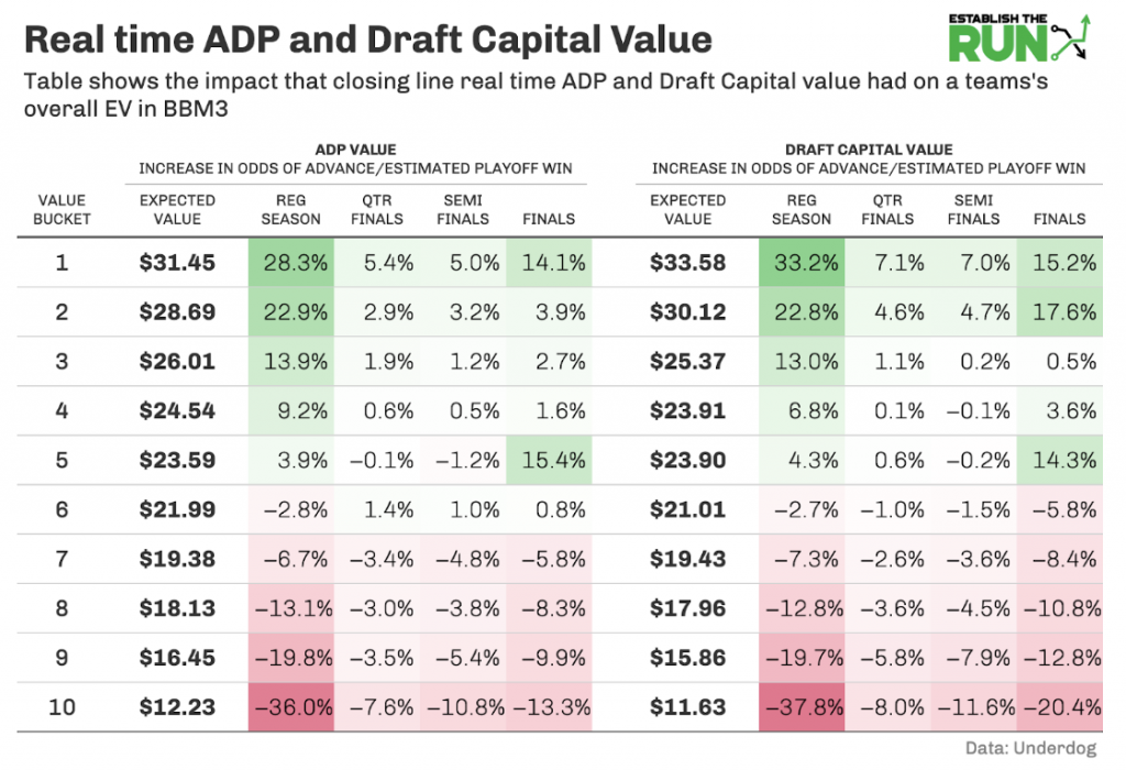
Let’s tie everything together to see how this affected the overall estimated EV of BBM entries.

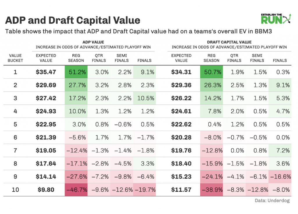
The optimal stack constructions we looked at in Part 2 led to EVs of $31.28 (two QBs rostered, both W17 game stacked) and $29.50 (three QBs rostered, all three W17 game stacked). Those figures are roughly similar to the average EV of being in a top-four bucket by either ADP Value ($29.40) or ADP Capital ($28.60) and worse than average EV of being in a top-two bucket by ADP Value or ADP Capital.

This is where I want to be clear about something. This is not a fair comparison. Structuring your team based on stacking is much more controllable than closing line ADP Value. I do believe achieving closing line ADP Value is a skill, but it’s not guaranteed at the time the draft closes. Stacking, on the other hand, is for the most part (sometimes players switch teams).

It is worth noting we didn’t have a ton of major offseason injuries last offseason that wildly impacted closing line value, and that you don’t even have to be in the very top of ADP Value to gain a meaningful EV edge. Those top four buckets that yielded great estimated EVs meant you just needed to be somewhere in the Top 40% among all drafted teams in that metric.

 

The three key takeaways for me are:

• • Stacking is more important than drafting for value because it’s a little bit more controllable at the time of the draft.
  • Getting closing line value on your draft picks can be just as important as having the right stack setup, sometimes even more so, in terms of impact on estimated EV.
  • You can see large increases in the EV of your BBM entries either through large increases in regular-season advance rate expectation OR increases in estimated playoff round win expectation.

 

It’s definitely fascinating to me how these two approaches can lead to similar EV:

• Gradual improvement in regular-season advance rate plus solid quarters and semis improvements plus big finals improvement (stacking)
• Large increase in regular-season advance rate plus gradual improvements in all playoff win rates (ADP Value)

 

Advance Rate VS Finals Win Rate

The above got me thinking: What exactly is the trade-off between regular-season advance rate and finals win rate?

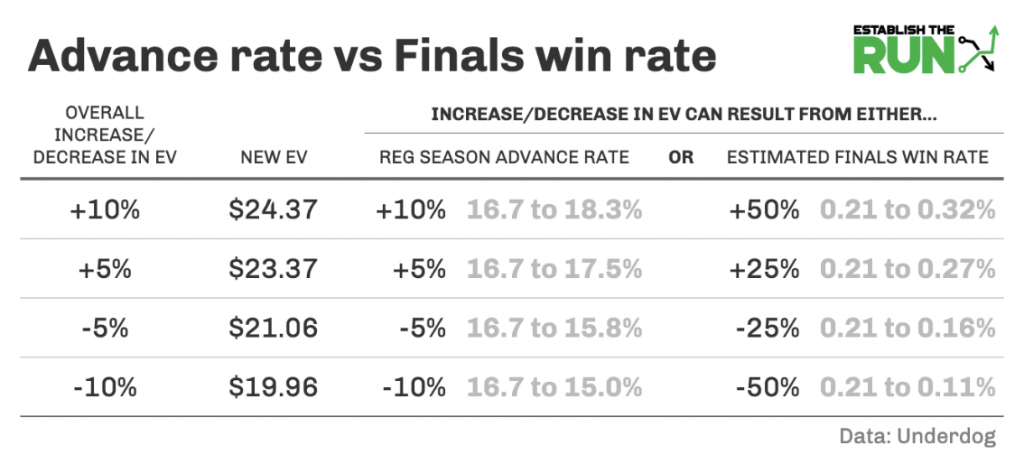
Now anyone could have done this analysis simply knowing the payout structure of BBM3, so I’m not trying to pass it off as novel, but for some reason, I never took the time to do the math before.

What we’re seeing above is that a 50% change in finals win rate is equivalent to a 10% change in regular-season advance rate in terms of impact on a team’s EV, which is essentially all we care about when we’re drafting. Keep in mind I am making some faulty assumptions in the EV calculation by assuming that all “losses” in each playoff stage receive the same payout. The true ratio may be a little smaller if you assume that increasing your finals win rate also increases your odds of any top-five finish, which is a reasonable assumption to make. As a result, a 4:1 ratio of finals win rate delta to regular-season advance rate delta may be a more responsible rough figure to keep in your head.

 

Number of “Live” Players

There are some elements of randomness that lend merit to trying to advance as many teams as possible regardless of playoff optimization. I don’t want to double-count here. In Part 1, when we compared 30 optimally stacked playoff teams versus 35 random playoff teams, the EV of the 35 random playoff teams already indirectly accounts for the analysis that is about to follow.

The primary element of randomness that I’m referring to is how many “live” players you have on your roster once you enter the playoff stages. This is something we have minimal control over, whether we stack or not, so your odds of running into a team with lots of “live” players increases with every additional team you have reach the playoff stages. What actual impact does that have?

For the analysis below, I am considering a “live” player as any player that scored more than zero points on a given week. This means a “dead” player could be an injured, suspended, or benched player.

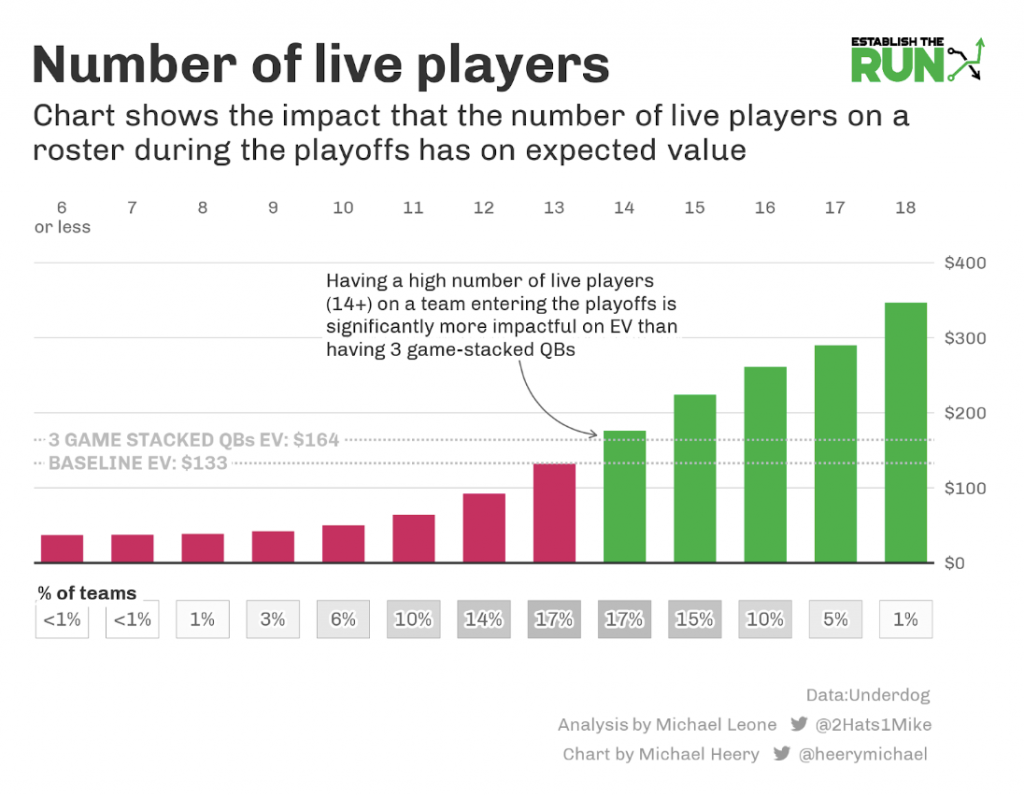
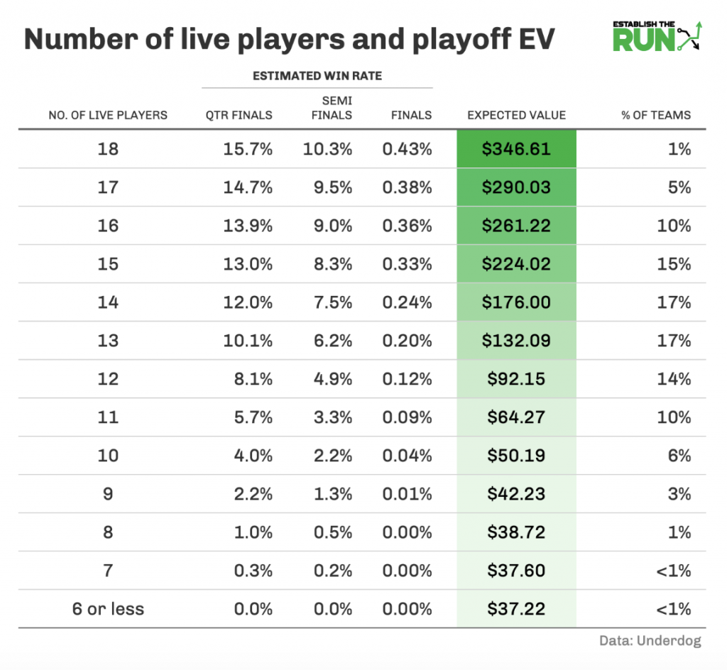
Notes:

• The EV shown above assumes a team makes it to the playoff stage in the first place.
• If you recall from Part 1, if looking purely at the number of game-stacked QBs, the highest playoff EV you could achieve was $164 with three game-stacked QBs.
• That number pales in comparison with the EV of a randomly constructed team that happens to have 14 or more “live” players for each of the playoff weeks.

 

The reason the number of “live” players is so impactful is worth spelling out, even if it seems obvious:

• First and foremost, the more “live” players you have, the less likely you’ve had an injury to important players you spent early draft capital on.
• Secondly, and to a much smaller degree, the more “live” players you have, regardless of draft capital spent, the more likely you’ll get lucky and run into a spike week or simply a necessary usable score on a given week.

 

We kind of saw this with Pat Kerrane’s winning BBM3 team. He had 15 “live” players, giving him 57% more likely odds than random of winning the finals week on that basis alone. Pat’s team avoided injuries to all of his significant players that he spent early draft capital on while receiving usable scores from picks in the double-digit rounds that were good enough to see the field (Raheem Mostert, Jakobi Meyers, and Tyquan Thornton).

So, while this is mostly the result of randomness, it’s worth keeping in mind in the back half of your drafts that you want a healthy mix of upside and uncertainty, as well as players that may be a bit more boring but are likely to hold onto any kind of role throughout the season.

 

Achieving ADP Closing Line Value

Coming back from the detour we took to look at the impact of “live” players, let’s return to how you can achieve ADP Value.

 

In drafts themselves, there are a couple of things you can do:

• Most obviously, being cognizant of current ADP when making your selections is likely to increase your odds of achieving final closing line value.
• Utilizing ETR ranks and thinking through the way the market is likely to adjust over the course of the draft season is somewhat subjective, but early draft season favorites of ours, such as Amon-Ra St. Brown and Chris Godwin, seemed very likely to see their ADPs rise as the draft season progressed.
• Embracing uncertainty. You can take shots on players with injury uncertainty (Chris Godwin, for example) and backup or rookie RBs. An injury in front of a backup RB can drastically change the backup’s ADP, as we saw with Darrell Henderson when Cam Akers got hurt two years ago. Taking shots on rookie RBs like Dameon Pierce last season prior to the chances of the preseason hype train to get going can also net you big ADP gains. You’re not going to be perfect in this regard, but given the above data, it’s worth considering when drafting.

 

There are two other components we control when it comes to drafting: when to draft and what type of draft (fast or slow) to choose. I think the common intuition of most drafters is that drafting early gives you more chances at achieving high closing line ADP value, but there’s also more risk of “dead players”. It’s also widely considered true that fast drafts are easier competition than slow drafts.

 

Time of Year

The following visuals show how frequently playoff teams had 13-18 “live” players in Week 15 from a given month.

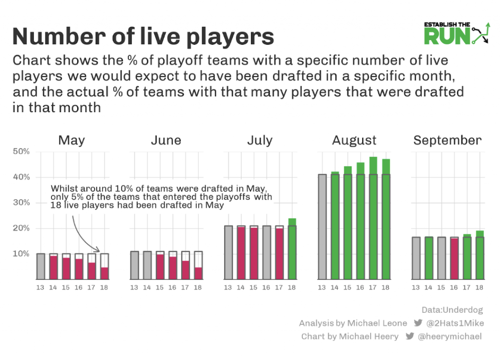
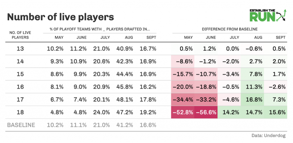
When I mention the number of live players from now on, I am specifically referring to the number of live players on Underdog teams in Week 15 that advanced to the playoff stages.

To clarify the visual above, 41.2% of all teams were drafted in August. So, if there was no correlation to the month when a team was drafted, we’d expect that 41.2% of all teams with 18 live players to have been drafted in August as well. However, 47.2% of teams with 18 live players were drafted in August. This means you were more likely to draft a team with 18 live players if you drafted in August than if you drafted in a different month.

 

The trend is quite clear:

• The earlier you draft, the less likely you are to make it to the playoff stages with 13+ live players.
• This impact is magnified as we look at the higher-end outcomes (15+ live players).
• July seems like a natural cutoff point. Teams drafted in May and June are fighting an uphill battle to get “lucky” and have a high number of live players. Teams drafted in August and September get a nice boost, but July is still fine.

 

Let’s do the same type of analysis for ADP Capital and see which months increase our odds of drafting a team with high-end ADP Capital.

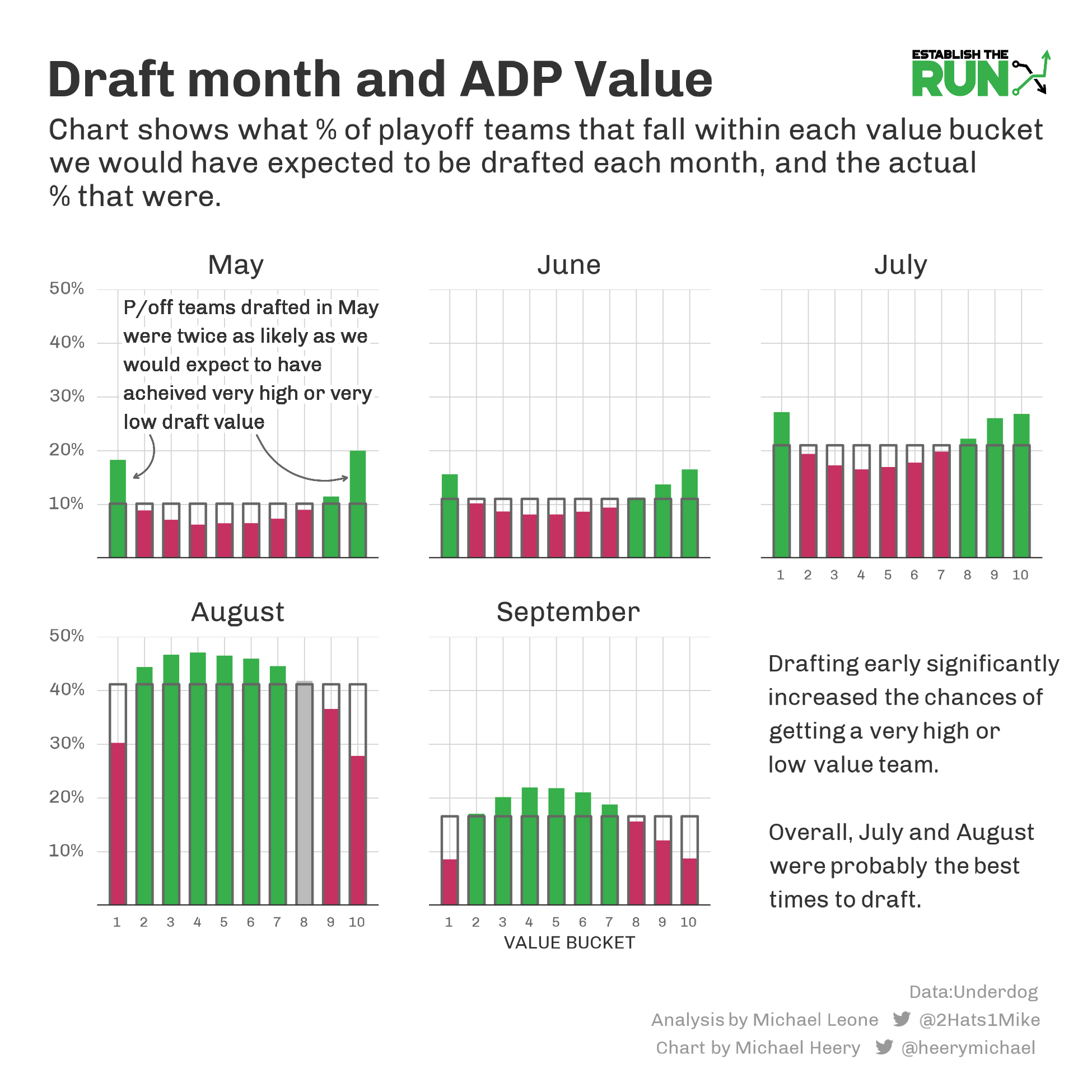
• Drafting early increases variance. Your odds of getting a very top team in terms of ADP Capital increase a lot in May, June, and July.
• The variance in May is particularly eye-opening, as the two biggest increases in likelihood are the ADP Capital bucket and the bottom. 
• You lose odds of having a top ADP Capital team in August, but if you look at Buckets 1-3 collectively (remember above that any team with a top-four ADP Capital bucket sees a nice increase in estimated EV), your odds only diminish slightly.

 

Putting it all together, I think the best time to draft is likely July and August. It’s purely anecdotal evidence, but it doesn’t hurt that Best Ball Mania 3’s $2 million winner (Kerrane), as well as the $1 million regular-season winner, both drafted on July 18.

Drafting somewhere between mid-July and mid-August seems to provide contestants with the best combined odds of achieving strong closing line ADP Value and having 13-plus live players on a roster when entering the playoff stages.

 

Fast versus Slow Drafts

I also wanted to look at your odds of achieving a good ADP Value based on fast versus slow drafts. Note that in the following analysis, I am looking only at drafts that Underdog marked as 30 seconds (fast) or 28800 (slow). There were some other clock types, likely from September when the clock changed, that I removed. This leaves us with 429,600 teams (95.2% of all teams) drafted with a traditionally slow or fast clock.

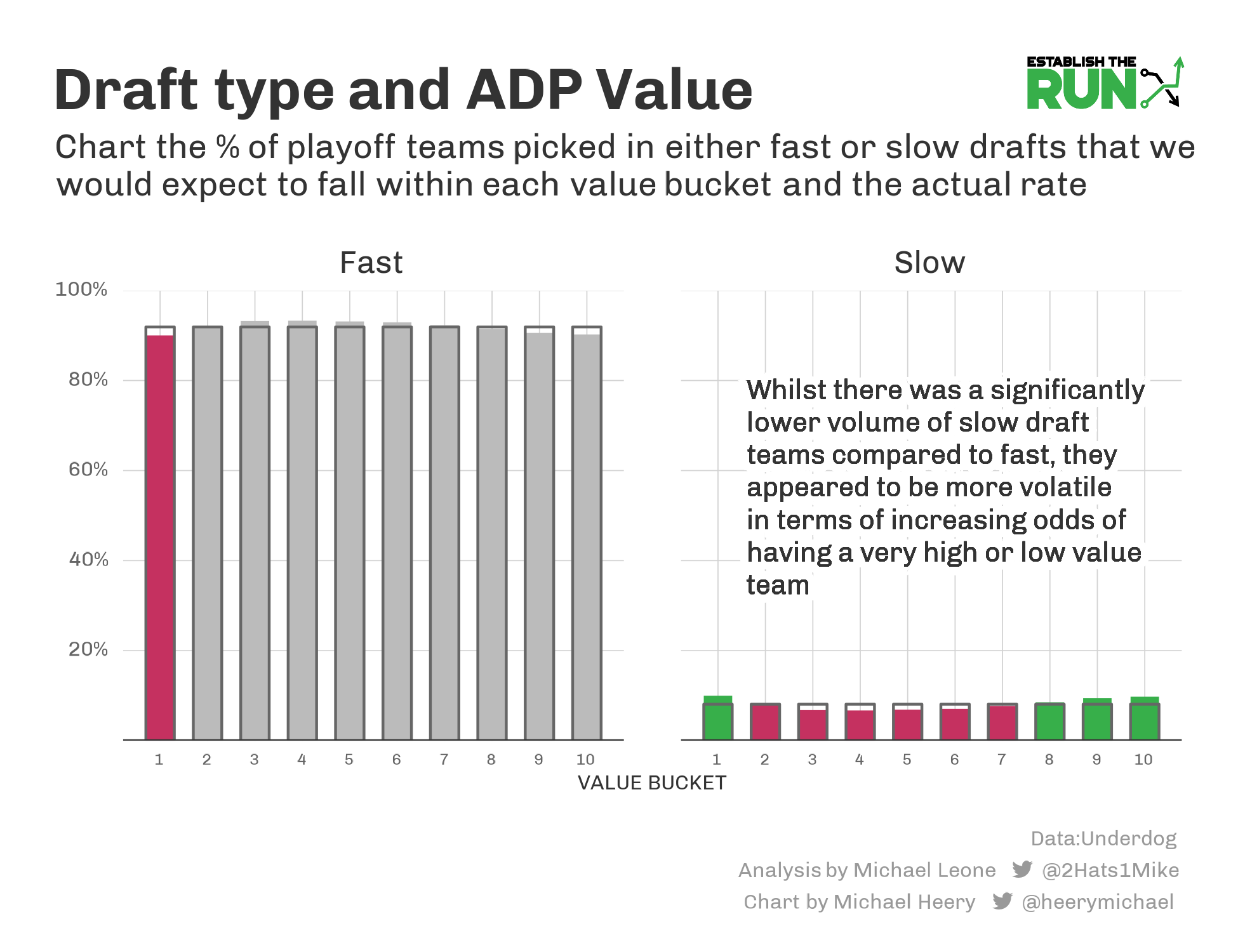
• At first glance, it seems like fast drafts have no edge in achieving ADP Value.
• On the other hand, slow drafts look quite volatile, expanding your odds of a very strong or very weak ADP Value.

 

However, we have a class imbalance. Slow drafts as a percentage of total drafts are weighted towards earlier in the offseason.

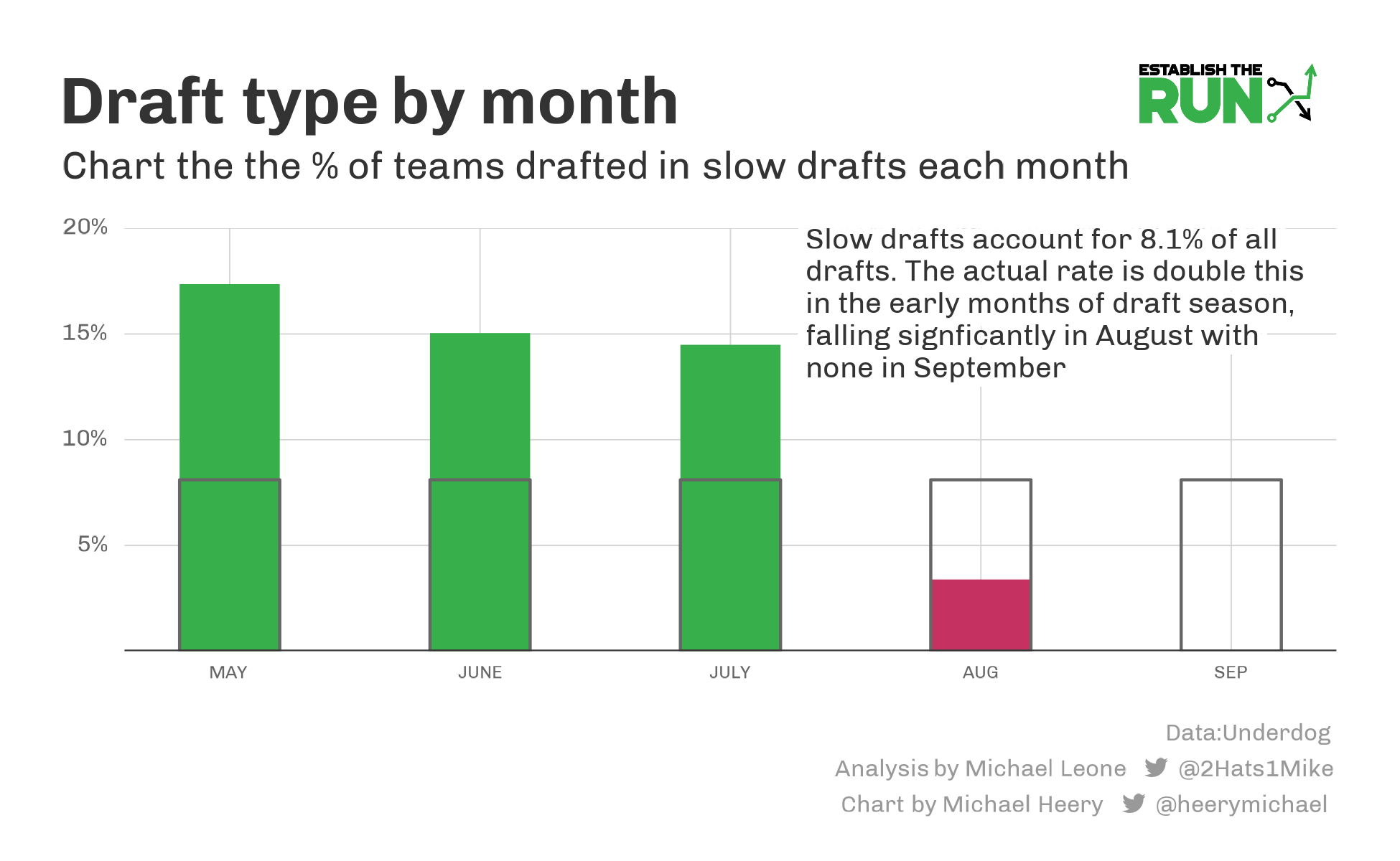
Sure enough, we see that while slow drafts comprise 8.1% of all drafts, that number is nearly doubled in May-July and minuscule in August-September.

When we account for the time of year slow drafts took place, we get a better picture of how they affect ADP Value:

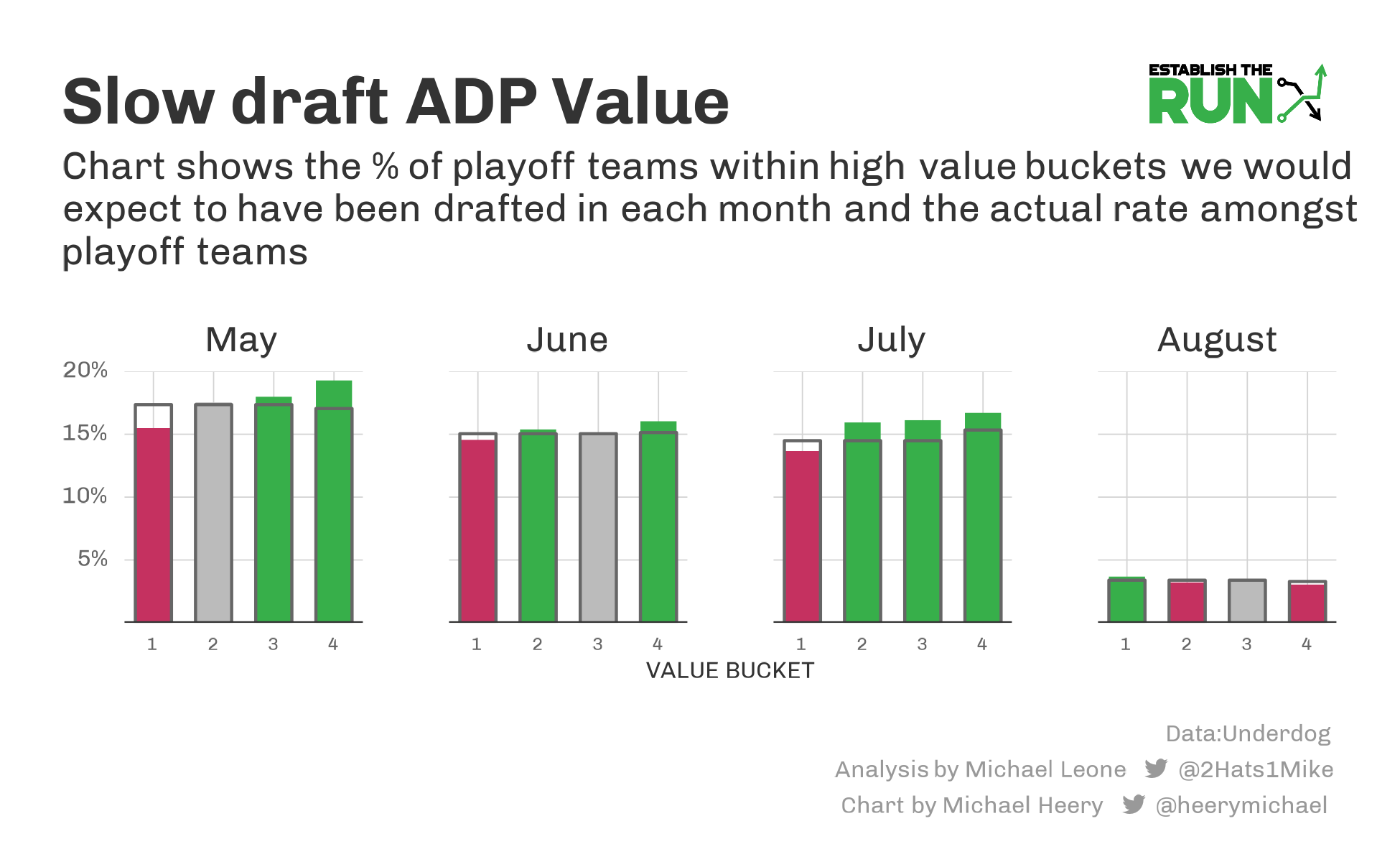
This chart compares the total percentage of slow drafts in a month to the total percentage of slow drafts that resulted in a specific ADP Value for that month. For example, in August, slow drafts represented 3.4% of all teams, but they represented 3.7% of teams with an ADP Value bucket of 1.

 

We see that:

• In general, slow drafts are only slightly worse than fast drafts in terms of ability to land in a top-three ADP Value bucket. From May to August, 9.8% of teams were drafted in a slow draft while 9.5% of teams in a top-three ADP Value bucket were drafted in a slow draft (a 2.6% decrease).
• This impact seemed most noticeable in May, where slow drafts as a percentage of teams saw a 10.8% decrease in representation among the top ADP Value bucket and a 4.4% decrease in representation among the top three ADP Value buckets aggregated together.
• It’s not a part of the image above, but when we modeled odds of advancing that included roster construction and ADP Value of all teams in the league, the data was similar. In other words, slow drafts seem slightly tougher than fast drafts, but it’s only a small difference.

 

Last season, I didn’t participate much in BBM3. It was difficult for me to carve out time for fast drafts, and I felt like I was losing too much EV participating in slow drafts. The data above I think shows that the general market sentiment that slow drafts are tougher is correct, but it’s a small magnitude. Personally, I’d rather do a fast draft than a slow draft for maximizing my EV, but unlike last season, I’m fine firing off a bunch of slow drafts if the decision is between a slow draft and not drafting.

 

Part 3: Roster Construction

In the past, we’ve looked at roster construction analysis by total rostered players at a position and the number of “early” draft picks at a position. This year, I replaced the “early” picks portion of the analysis with draft capital spent, as I think it’s a more flexible metric, rather than one with an arbitrary cutoff (first five rounds) that does not capture much nuance (first-round pick treated the same as a fifth-round pick).

I discussed the concept of draft capital in Part 2 of this article, but essentially I used a quick model to give each pick in the draft a draft capital equivalent based on the average expected points above replacement player that pick provided.

Here’s the chart for draft capital, from pick 1 to pick 216:

For each position, I will look at the combination of total draft capital spent at the position and the total number of players rostered at the position and how that impacted regular-season advance rates and estimated playoff win rates. For draft capital spent, I split positional spending into five buckets. Bucket 1 is the most spending (80th-100th percentile), while Bucket 5 is the least amount of spending (0-20th percentile).

 

Caveats

The estimated playoff win rates do not factor in the three uncorrelated playoff stages (quarterfinals, semifinals, and finals) being played in consecutive weeks with a lot of correlation between rosters. So, there are elements my analysis doesn’t capture. For example, having three QBs may be more favorable than the data suggests in such a format. Also, Zero RB may help provide a uniqueness boost to teams that advance deep (more likely to run into a projected RB1 on a given week that isn’t rostered heavily elsewhere). I’m not sure if either of the previous two statements are accurate, but these are ideas sharp players should consider in a format like Best Ball Mania.

Also, my use of “optimal” in this article, and especially in this section, may be misleading. More than anything else, the analysis below is a description of what happened in general last season. There are well-drafted teams that may not tick the boxes of what was optimal at each of the positions last year, and Pat Kerrane’s $2 million winning team is evidence of that. That’s in large part due to the fact that:

• What was optimal in retrospect can largely be influenced by outlier seasons, good or bad, by individual players.
• Quality overall roster construction is more about logically layering together different strategies and correctly balancing your capital allocations, which is more of a dynamic equation based on your specific draft than it is trying to force everything you do to fit neatly and tidily into the cohort analysis that follows.

Travis Kelce at TE, Jalen Hurts at QB, Justin Jefferson at WR, and Josh Jacobs at RB had such outstanding and impactful seasons. In some ways, the following analysis is a repackaged way of telling us just that. When you get to the TE position, it’s clear the impact a single player (Kelce) had on the results.

I still think it’s important to understand exactly what worked last season, in what way, and why, but as I will consistently remind readers throughout Part 3, you need to think critically when taking these results and applying them to next season.

 

Quarterback

Regular Season

QBs Rostered and Draft Capital Spent (Individually)

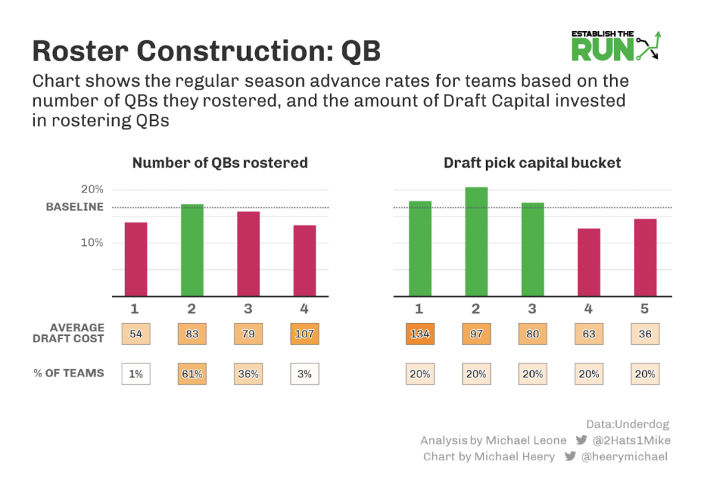
• Rostering two QBs in general is better than rostering three QBs.
• Rostering anything but two or three QBs is a bad idea.
• You cannot skimp on spending at the QB position.
• The second-tier spending had an amazing hit rate.

 

QBs Rostered and Draft Capital Spent (Combined)

 

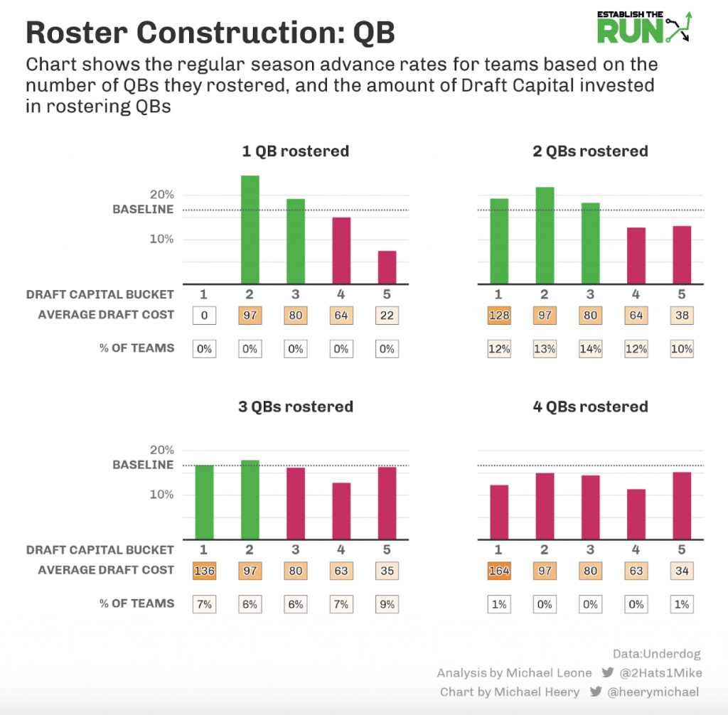
• Not surprisingly, the combination of rostering two QBs and spending in that second tier of QB draft capital provided by far the best advance rate.
• Hero QB was actually okay in terms of advance rate if the QB was a very early pick. If you recall from Part 1, I showed that the EV of a Hero QB team was poor despite a good estimated finals win rate because of low advance rates (more on this in the playoff section).
• I was surprised to see there wasn’t a combination of three QBs rostered and a particular draft capital bucket that increased advance rates. Again, the specific QB outcomes of the season are driving this, but even among 3-QB teams, you wanted to be in that second tier of draft capital spent.
• It really doesn’t ever make sense to draft four QBs, but if you’re going to try it, you might as well get them all late.

 

To provide more context to the visual you’re seeing above, let’s look at several examples from each QB Bucket in terms of draft capital spent:

 

2 QBs

QB Bucket 1: Justin Herbert (44) and Jalen Hurts (68)

QB Bucket 2: Russell Wilson (68) and Kirk Cousins (116)

QB Bucket 3: Kyler Murray (55) and Jared Goff (199)

QB Bucket 4: Tom Brady (76) and Zach Wilson (143)

QB Bucket 5: Derek Carr (105) and Matt Ryan (153)

 

3 QBs

QB Bucket 1: Patrick Mahomes (54), Dak Prescott (91), and Matt Ryan (163) 

QB Bucket 2: Derek Carr (87), Kirk Cousins (111), and Matt Ryan (154)

QB Bucket 3: Lamar Jackson (52), Jameis Winston (173), and Baker Mayfield (196)

QB Bucket 4: Trey Lance (86), Zach Wilson (134), and Carson Wentz (203)

QB Bucket 5: Daniel Jones (136), Carson Wentz (177), and Davis Mills (201)

 

As an example of why the above information is important to learn from but not to blindly replicate, Pat Kerrane pretty intentionally married a 3-QB strategy with an elite early RB strategy. Additionally, Kerrane stacked all three of his QBs with at least one pass catcher and Week 17 game stacked two of his three QBs, something we saw in Part 1 was critical in improving the overall EV of his team.

Kerrane actually ended up in the 3-QB, QB Bucket 4 segment that had a horrible regular-season advance rate. This doesn’t mean he messed up the QB position. You need to think critically based on your specific draft landscape, the specific players you’re taking, and the specific construction you’re building out across all positions. While I don’t believe this is the case with Kerrane’s team, the flip side of this is also: Just because someone wins does not always mean their strategy was correct.

 

Here’s Kerrane’s QB draft:

3-QB, QB Bucket 4:

Tom Brady (90), Tua Tagovailoa (138), and Daniel Jones (162)

 

Another note on his construction is that Kerrane got positive ADP Value on his trio of QBs. If we look at draft capital spent by final ADP instead of actual pick, Kerrane is at 70.7. The average draft capital spent by final ADP for the 3-QB, QB Bucket 4 group was much lower at 60.9.

This might seem obvious, but you can spend less draft capital on that position if you’re getting good value on that position. And there’s further room to layer in how you like the players subjectively. For example, by ETR positional value, Tom Brady was ETR’s QB9 (QB10 by ADP), Tua Tagovailoa QB16 (QB17), and Daniel Jones QB19 (QB21).

Kerrane had a more beefed-up QB room than his pick draft capital suggests, and he layered it with the correct complementary strategies (early RB without sacrificing WR quantity, swing at an elite TE, and stacking optimization).

I hope that little detour analyzing Kerrane’s specific QB draft helps you to mesh the macro trends that are important to understand with the notion that you’re going to have to think critically and be flexible in your actual draft to optimize your teams, especially given that this data can be moot based on your competitors and ADP changes.

 

Playoffs

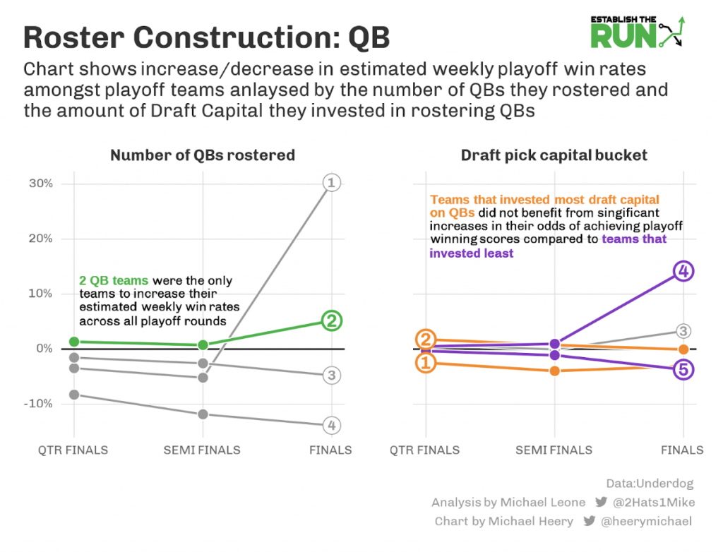
• Estimated playoff win rates are more or less unaltered by QB structure. 
• Taking four QBs is clearly bad. 
• Being on the extreme ends of draft capital spent is slightly -EV.

 

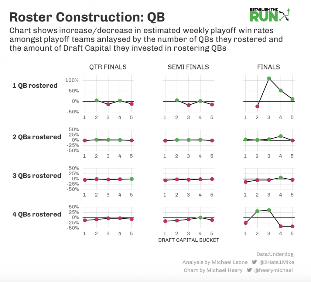
• Like when we looked at the pieces individually, there’s not much movement in terms of estimated playoff win rates based on QB structure.
• It’s somewhat fascinating that our intuition on elite QB for last season at least was wrong. Investing in elite QBs had a clear edge in improving regular-season advance rates, but, for whatever reason, that did not translate to any meaningful improvement in the single-week upside needed to win the playoff stages.

 

Expected Value

Combining the above analysis on regular-season and estimated playoff win rates, we can derive an overall EV (Expected Value) for teams based on their combination of the number of QBs and QB draft capital spent bucket.

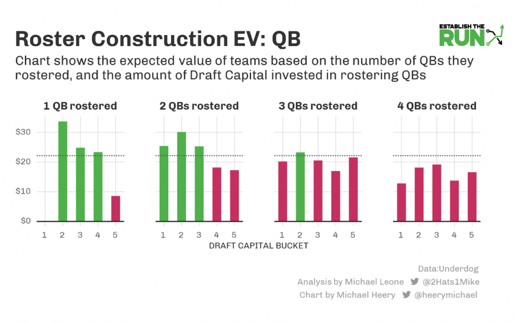
• A few of the Hero QB teams spit out a solid estimated EV. This is very noisy due to sample size, and I remain skeptical that this is a valid strategy when you layer in the reduced outs in terms of stacking potential and surviving three straight uncorrelated tournaments with a single QB.
• 2-QB teams and the second QB Bucket both pop as the highest EV strategies overall, but this is mostly influenced by changes to regular-season advance rates given the minimal impact of QB structure on estimated playoff win rates.

 

Running Back

Regular Season

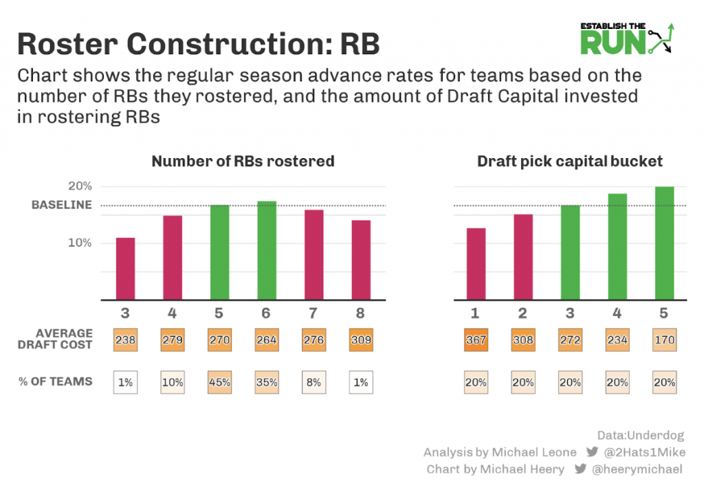
• The less draft capital a team spent on the RB position, the higher their likelihood of advancing in the regular season.
• It’s interesting to see that the field was pretty sharp in terms of adjusting draft capital based on the number of RBs selected. Teams that took only three RBs were light on capital spent, and teams that took eight RBs were heavy on capital spent (on average). However, teams selecting between four and seven RBs spent on average the same total draft capital on the position (273), which is right in line with the middle bucket of RB draft capital spending.
• The extremes (three or eight RBs selected) were poor strategies.
• Taking five or six RBs total, which was by far the two most popular allocations by the field, had the clear best advance rates.

 

Now let’s look at the combination of total RBs rostered and total RB draft capital spent (minimum 1,000 teams):

 

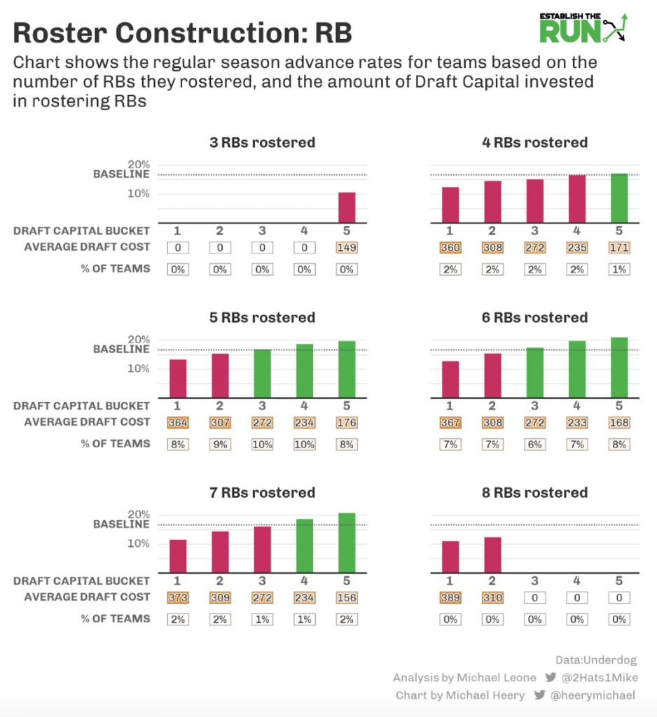
• While five and six RBs rostered was centered on by the field, how teams allocated total draft capital within those builds was pretty spread out.
• No matter how many RBs a team rostered, their advance rate increased if they allocated less draft capital to the position. This was even true for HyperFragile teams (four RBs).
• Teams that took seven RBs had difficulty keeping their total RB draft capital spent in check, but those that did (RB Draft Capital Buckets 4 and 5) saw advance rates similar to the 5- and 6-RB teams.

 

Playoffs

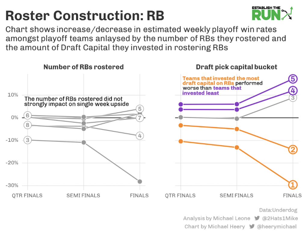
• The impact is less steep, but like with the regular season, teams that spent less RB draft capital had the highest estimated playoff win rates.
• The impact of the quantity of RBs made less of a difference, with the exception of 3-RB teams and to a lesser extent 4- and 8-RB teams.

 

 

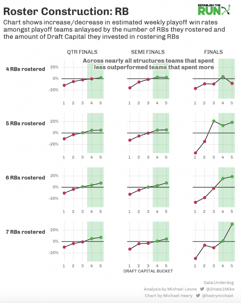
• Combining RBs rostered and RB draft capital spent paints more of the same picture: It was a bad year to overinvest in the RB position.
• Same as in the regular season, the 7-RB strategy pops as a real weapon when total RB draft capital spent is managed correctly.

 

EV Estimate

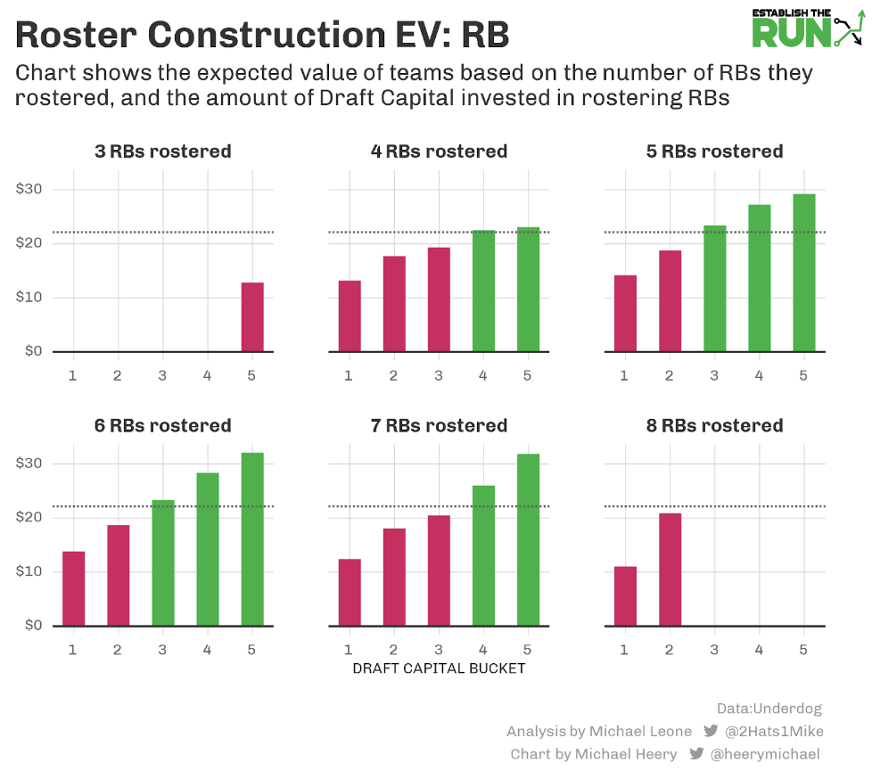
As we did at QB, let’s look at some examples of actual RB constructions so it’s easier to get a feel of what the above combinations look like in practice:

 

4 RBs

Bucket 1: Derrick Henry (9), Joe Mixon (16), James Conner (33), Dameon Pierce (136)

Bucket 2: Dalvin Cook (7), Aaron Jones (18), Tony Pollard (103), Tyler Allgeier (138)

Bucket 4: Austin Ekeler (6), Rashaad Penny (102), Cordarrelle Patterson (115), Alexander Mattison (126)

Bucket 5: Ezekiel Elliott (52), Dameon Pierce (69), Tony Pollard (76), Eno Benjamin (196)

 

5 RBs

Bucket 1: Joe Mixon (13), Ezekiel Elliott (36), A.J. Dillon (60), Chase Edmonds (85), Khalil Herbert (156)

Bucket 2: Dalvin Cook (9), A.J. Dillon (57), Chase Edmonds (81), Clyde Edwards-Helaire (88), Miles Sanders (112)

Bucket 4: Alvin Kamara (29), Travis Etienne (44), Damien Harris (101), Dameon Pierce (140), Darrel Williams (164)

Bucket 5: Breece Hall (40), A.J. Dillon (81), Kenneth Walker (105), Rhamondre Stevenson (129), Trey Sermon (208)

 

6 RBs

Bucket 1: Dalvin Cook (11), D’Andre Swift (14), J.K. Dobbins (59), Nyheim Hines (134), Kenneth Gainwell (158), Jerick McKinnon (203)

Bucket 2: Jonathan Taylor (1), Leonard Fournette (25), Rhamondre Stevenson (73), Brian Robinson (169), Jeff Wilson (193), Sony Michel (216)

Bucket 4: Aaron Jones (20), Josh Jacobs (77), Clyde Edwards-Helaire (92), Cordarrelle Patterson (101), Raheem Mostert (173), Samaje Perine (212)

Bucket 5: Javonte Williams (30), Samaje Perine (102), Rachaad White (115), Kenneth Walker (126), Alexander Mattison (139), Michael Carter (163)

 

7 RBs

Bucket 4: Christian McCaffrey (2), Kenneth Walker (95), Kareem Hunt (98), Darrell Henderson (122), Tyler Allgeier (146), Raheem Mostert (191), Jeff Wilson (215)

Bucket 5: Breece Hall (54), Travis Etienne (67), James Cook (126), Khalil Herbert (150), Brian Robinson (163), Zamir White (174), Tyrion Davis-Price (187)

 

Kerrane’s winning team was a 5-RB, RB Bucket 3 team that got a ton of closing line value: Austin Ekeler (7), Saquon Barkley (18), Rhamondre Stevenson (114), Raheem Mostert (186), Sony Michel (199)

 

Closing Line ADP Value

The RB results are drastic and consistent, so let’s try to understand them a bit more. Digging deeper, we see that there’s a link between closing line ADP Value, the importance of which was detailed in Part 2, and RB allocation.

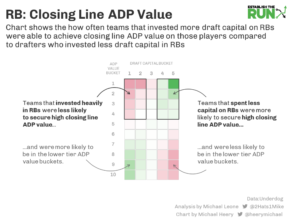
• Teams who spent more on RB draft capital were about 13% less likely to be in the top 20% of ADP value and 13% more likely to be in the bottom 20% of ADP Value.

• Teams who spent the least on RB draft capital were 27% more likely to be in the top 10% of ADP Value and 12% less likely to be in the bottom 20%.

 

This is essentially the whole point of Zero RB, which I’ve been skeptical of overly applying to Underdog in the past. Because this is a position where volume and role are so heavily correlated to value, we see more variance in ADPs across the contest. This, of course, also extends to variance in regular-season value.

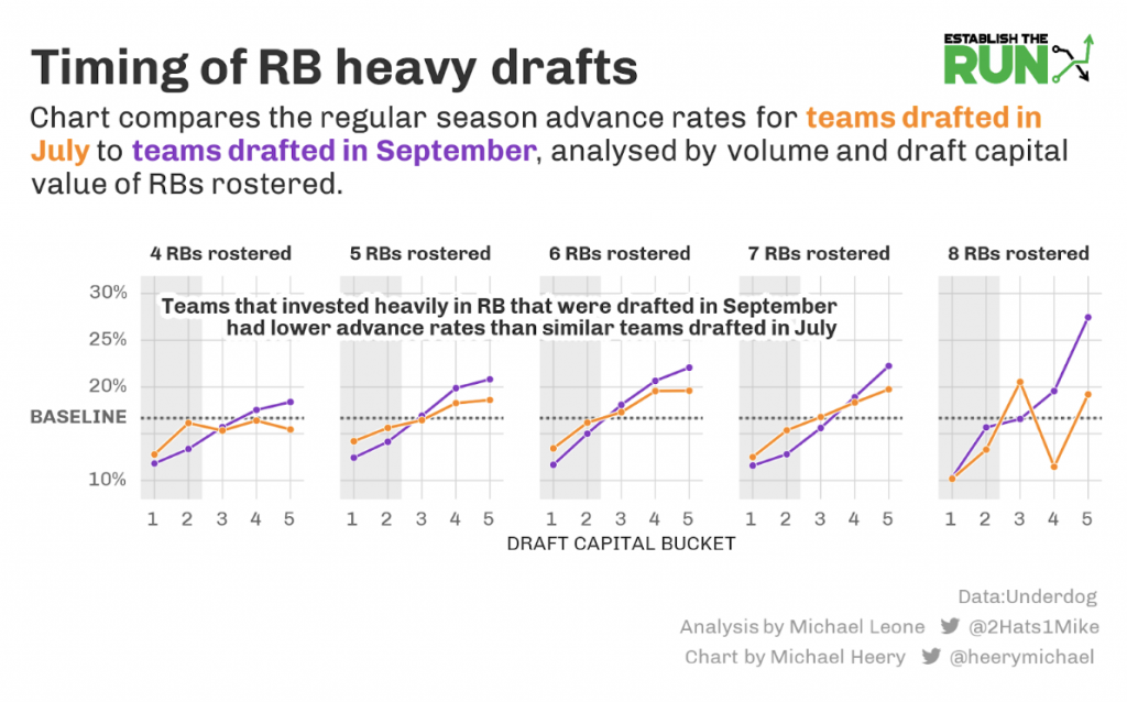
I thought that this might mean that teams drafting earlier in the offseason should be more slanted to Zero RB, but if we compare September drafts to July drafts, we actually see that spending more on RB draft capital is worse in September.

Positional Scarcity

I recently had Sam Sherman on a podcast to talk about some misconceptions between RB and WR production, predictability, and flex scoring on my Establish the Edge Podcast.

Essentially, Sam’s data shows that RBs contribute just as much to the flex as WRs and that RB spike weeks are just as common as WR spike weeks, even after accounting for ADP.

Yet, we’re seeing such a strong negative correlation between RB investment and team success.

As we’re seeing above, the link between RB investment and closing line ADP value is one reason, but since it’s not overly shaped by the time of year, there has to be something else going on.

Sam and I surmised it may just come down to boring old position scarcity.

Let’s take a deeper look at that.

Assuming that 90% of the time the flex is filled by an RB or WR on Underdog and that it is split equally between the two positions, we arrive at 3.45 starting WRs and 2.45 starting RBs. In theory, that ratio (3.45:2.45 or 1.4:1) should be reflected in how teams spend their draft capital.

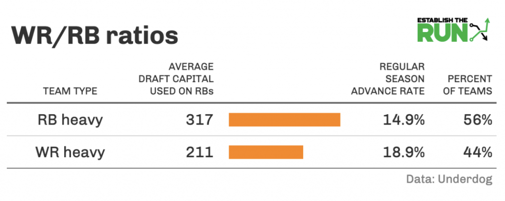
What we see is twofold:

• The field is playing too many RB-heavy teams if you assume the 1.4:1 ratio is correct (55.6%).
• The 1.4:1 ratio is not correct. RB-heavy teams are performing much worse than WR-heavy teams using that as the breakeven point.

 

Carving up the WR:RB ratios into 20th-percentile buckets as we did with positional draft capital, we don’t really see any convergence on the “expected” ratio:

It’s important to keep in mind this is based on just a single year, but there are a few elements working together:

• Zero RB strategies are working on Underdog.
• RB is one of the easier positions to gain closing line ADP value on, so it makes sense to not overinvest in the position early.
• The field isn’t properly accounting for positional scarcity.

 

Wide Receiver

Regular Season

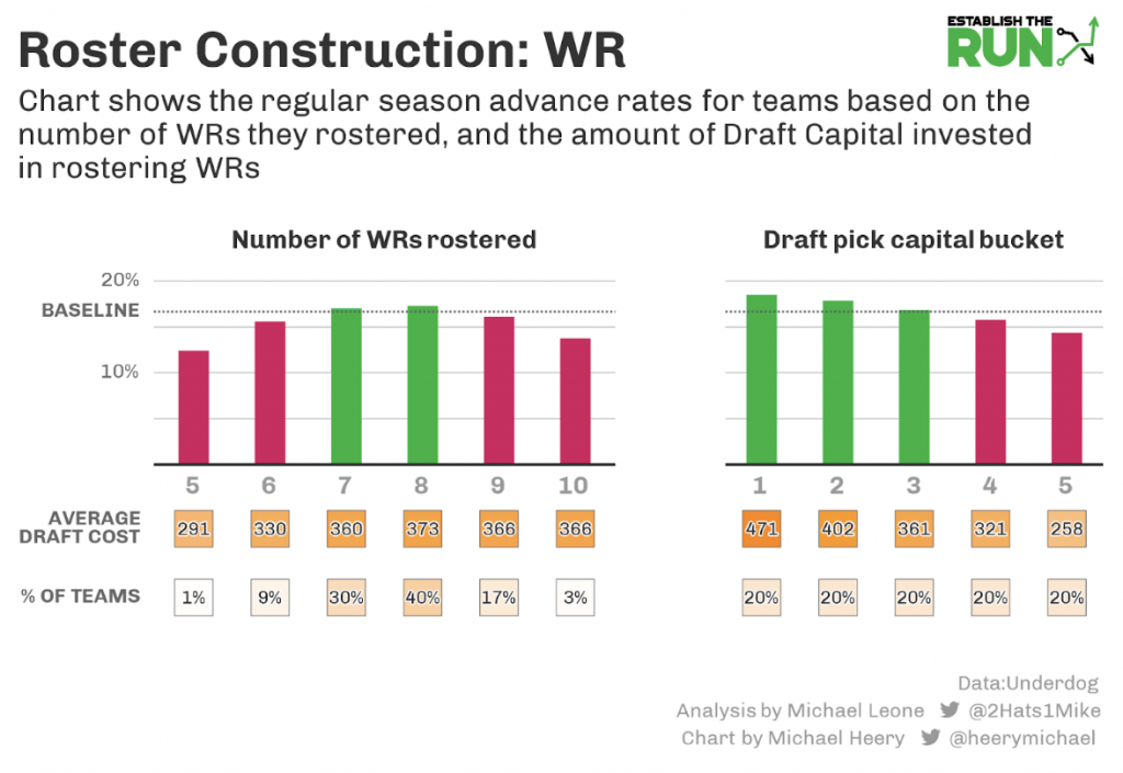
• These things tend to pivot off of each other, so it’s logical given the RB results, but the more you invest in WR, the better your advance rates.
• Super high-quantity WR teams fared poorly last season (hand in hand with HyperFragile not doing so well).
• There weren’t huge differences between taking 6-9 WRs, but seven and eight WRs were most optimal last season.

 

Now let’s look at the combination of total WRs rostered and total WR draft capital spent (minimum 1,000 teams):

 

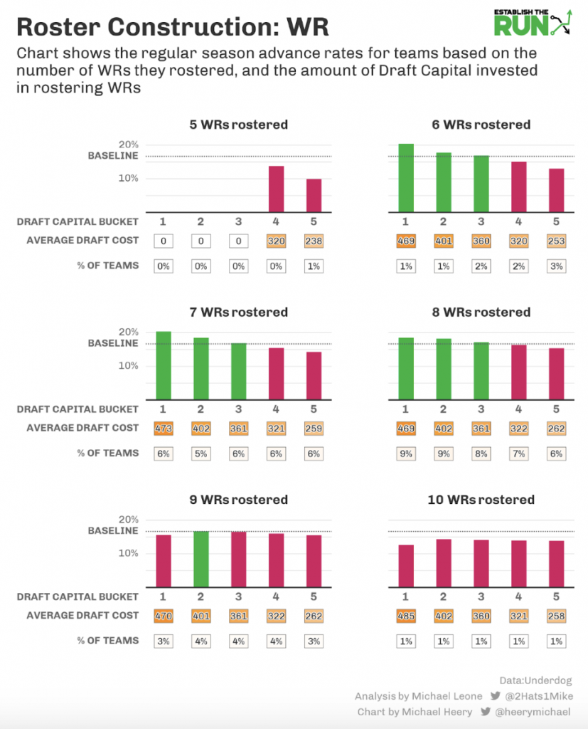
• The fewer WRs you take, the more important it is to invest premium draft capital into the position. In fact, the only combinations to eclipse a 20% advance rate were six and seven WRs rostered paired with Bucket 1 WR spending.
• 9-WR teams that had middle-of-the-road overall WR spending fared the best.

 

It’s important, again, to note how the individual player outcomes shape the overall roster construction, making it somewhat noisy from year to year. If early WRs perform really well, then the teams that took those WRs and fewer WRs total are going to have good rates. Flowing from that, those teams are naturally aligned with teams that spent less at RB but rostered higher quantities of RBs.

6- and 7-WR teams did fare well last season, too, and I think I need to be more open to those types of builds. It’s generally a mental barrier I have a tough time overcoming to only draft six WRs. Two seasons ago, quantity over quality at WR was more successful. It’s difficult to tell if that doesn’t work as well anymore as WR ADP gets pushed up at all points of the draft, or if we will see a resurgence for that strategy.

I’m being repetitive as I’ve made this point directly as it relates to Kerrane’s winning team already, but the big takeaway here is:

• Meshing complementary strategies is important.
• It’s good to be aware of what worked in the previous season and why so you can decide if it makes sense to mimic those strategies again in 2023 or if there’s an opportunity to deviate. When Best Ball Mania 4 is released, I hope to do some content that’s a bit more forward-looking in terms of how we should be building specifically for this season with that contest structure and the current draft landscape.

 

Playoffs

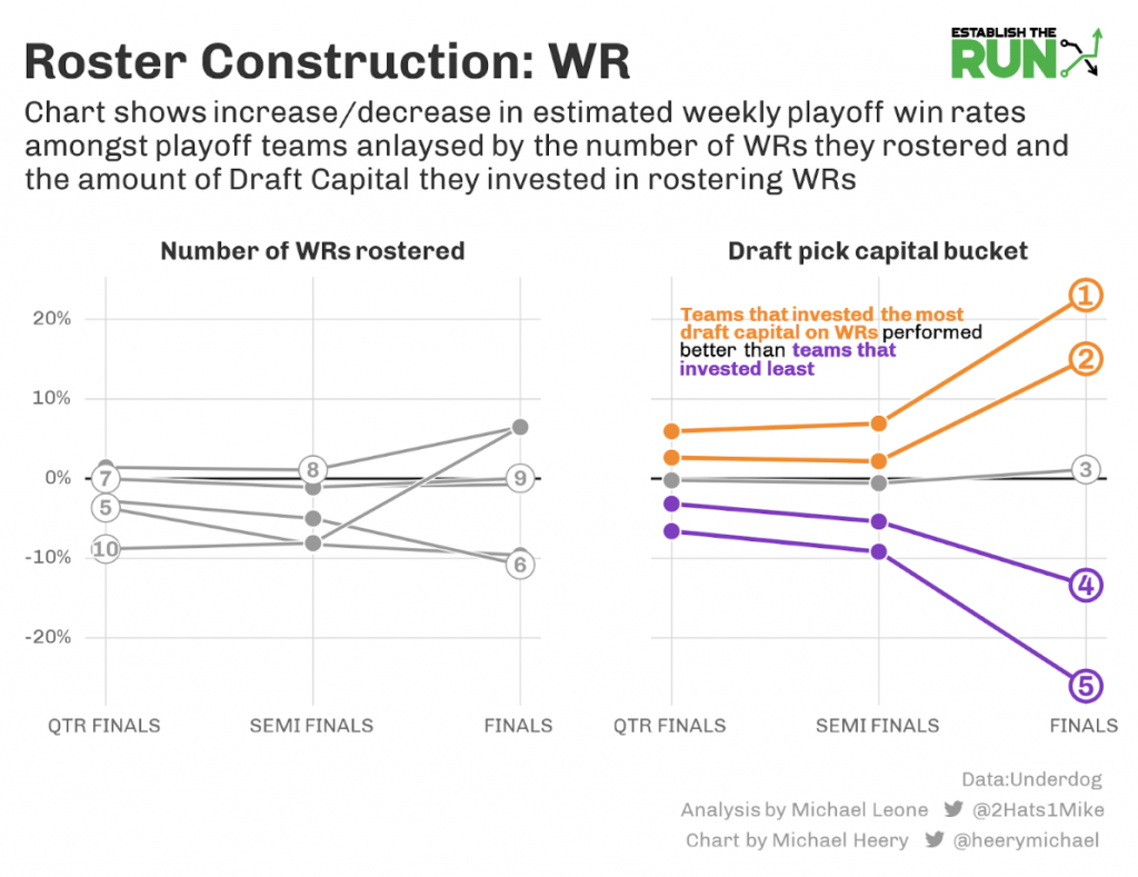
• As with most of the roster construction segments, the impact on estimated playoff win rates is a lot tamer than it is for regular-season win rates.
• WR spending translates well from regular-season success to playoff success.
• However, the quantity of WRs becomes less impactful, and the 6-WR teams start to fare a bit worse. Rostering 7-9 WRs is best in terms of estimated playoff win rates.

 

 

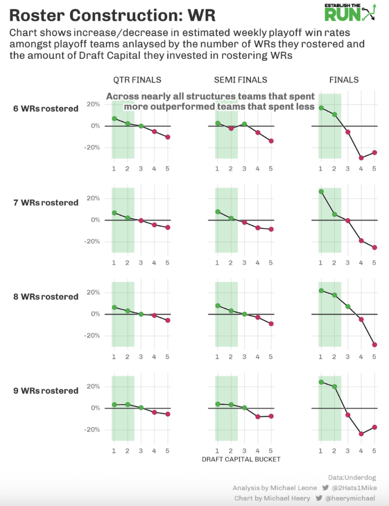
• 6-WR teams look better in the playoffs when you isolate them to the ones that spent the most on WR draft capital. Ironically, more of the field that was rostering six WRs spent less on draft capital than they should have.
• The 9-WR teams that performed the best in the playoffs were still spending a lot of total capital on the position.
• 10-WR teams had some strong finals win rates but struggled in the smaller-field stages.

 

EV Estimate

 

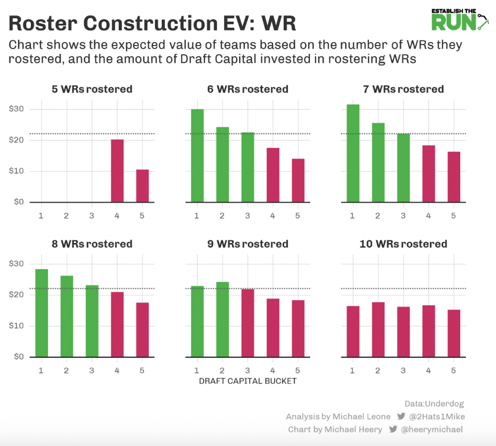
Let’s take a look at what some of these WR builds look like in action:

 

6 WRs

Bucket 1: Justin Jefferson (3), A.J. Brown (22), Mike Williams (25), Jaylen Waddle (46), Allen Robinson (51), Brandon Aiyuk (94)

Bucket 3: Tyreek Hill (23), A.J. Brown (26), Amon-Ra St. Brown (50), Chris Olave (95), Josh Palmer (122), Michael Gallup (143)

Bucket 5: D.J. Moore (32), Jerry Jeudy (56), DeVonta Smith (80), Hunter Renfrow (89), Chase Claypool (113), Will Fuller (200)

 

7 WRs

Bucket 1: Ja’Marr Chase (5), Mike Evans (20), Michael Pittman (29), Allen Lazard (68), DeAndre Hopkins (77), Marquez Valdes-Scantling (92), Tyquan Thornton (197)

Bucket 3: D.J. Moore (32), Terry McLaurin (41), Brandon Aiyuk (65), Skyy Moore (89), Robert Woods (104), Rondale Moore (113), Laviska Shenault (200)

Bucket 5: Keenan Allen (25), Amon-Ra St. Brown (48), Tyler Lockett (97), Garrett Wilson (121), Jakobi Meyers (145), Christian Watson (168), Wan’Dale Robinson (169)

 

8 WRs

Bucket 1: Ja’Marr Chase (5), Tyreek Hill (20), Terry McLaurin (44), Rashod Bateman (53), Mecole Hardman (125), Wan’Dale Robinson (164), Parris Campbell (173), Devin Duvernay (212)

Bucket 3: Courtland Sutton (35), Gabriel Davis (38), Darnell Mooney (62), Kadarius Toney (86), Tyler Lockett (107), Isaiah McKenzie (131), Marvin Jones (179), Parris Campbell (182)

Bucket 5: DK Metcalf (56), Brandon Aiyuk (65), Chris Olave (89), Tyler Lockett (104), Chase Claypool (113), Rondale Moore (128), Sammy Watkins (185), Zay Jones (200)

 

9 WRs

Bucket 1: Justin Jefferson (5), Jaylen Waddle (44), Gabriel Davis (53), Amon-Ra St. Brown (77), Treylon Burks (92), Kenny Golladay (116), Mecole Hardman (125), Jalen Tolbert (149), Wan’Dale Robinson (188)

Bucket 3: Stefon Diggs (7), Deebo Samuel (18), Drake London (79), Tyler Boyd (114), Jahan Dotson (127), Robbie Anderson (151), Marvin Jones (175), Odell Beckham (199), A.J. Green (210)

Bucket 5: Jaylen Waddle (37), Michael Thomas (60), Chris Godwin (61), Treylon Burks (109), DeVante Parker (156), Cedrick Wilson (180), Kenny Golladay (181), Devin Duvernay (204), Erik Ezukanma (205)

 

Kerrane was in WR Bucket 3 with eight WRs rostered:

D.J. Moore (31), Jaylen Waddle (42), Chris Godwin (66), Hunter Renfrow (79), Tyler Lockett (103), Jakobi Meyers (127), Wan’Dale Robinson (175), Tyquan Thornton (210)

 

Tight End

Regular Season

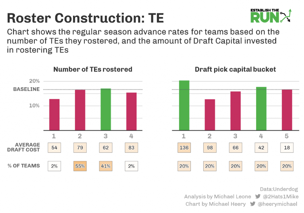
• So much of this is driven by Travis Kelce smashing (he represents a large portion of the Bucket 1 teams) and Kyle Pitts failing (Bucket 2 teams).
• Taking two or three TEs in general netted the best regular-season advance rates.

 

• The one TE rostered segmentation is interesting. Basically, if you get a Kelce-type season, just taking one TE can be really beneficial.
• However, if you don’t get a Kelce-type season, you’re battling steeply uphill.
• The two and three TEs rostered are so shaped by Kelce >>> all the other early-drafted TEs, but in general, the trend was to either spend way up at TE or else be middle of the pack.
• 4-TE teams are generally -EV, but if you’re going to do them, you want to spend as little overall capital on the position as possible.

 

Playoffs

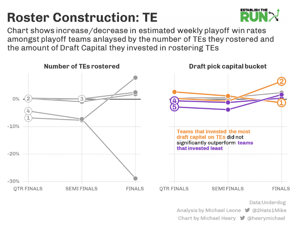
• Four TEs are brutal in the playoff stages.

 

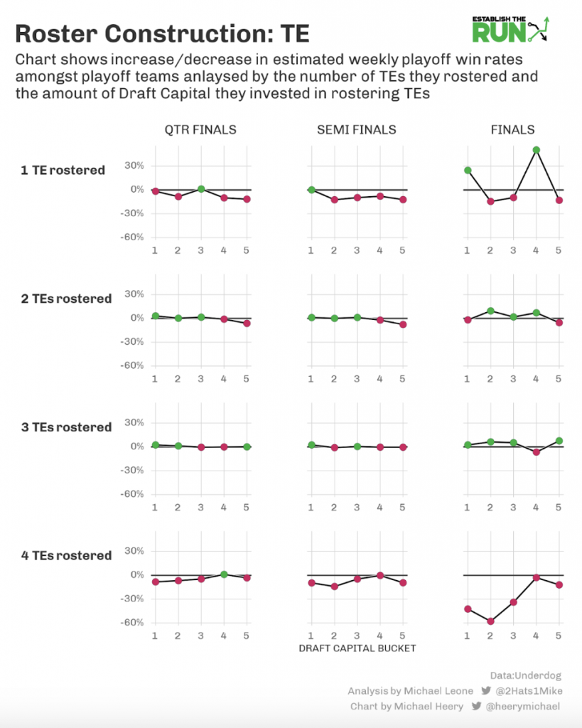
• Hero TE remains viable in the playoffs with a Kelce-type season.

 

EV Estimate

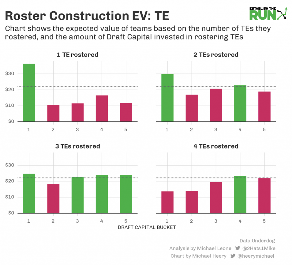
• I don’t know if you noticed this, but Travis Kelce had a good season last year and that impacts the results.

 

1 TE

Bucket 1: Travis Kelce (15)

 

2 TEs

Bucket 1: Travis Kelce (15), Tyler Higbee (183)

Bucket 2: George Kittle (56), Albert Okwuegbunam (156)

Bucket 4: Robert Tonyan (132), Irv Smith (133)

 

3 TEs

Bucket 1: Kyle Pitts (29), Pat Freiermuth (140), Tyler Higbee (164)

Bucket 2: T.J. Hockenson (82), Zach Ertz (111), David Njoku (178)

Bucket 4: Dawson Knox (104), Hayden Hurst (185), Cameron Brate (209)

Bucket 5: Irv Smith (149), Austin Hooper (188), Jonnu Smith (212)

 

4 TEs

Bucket 1: Mark Andrews (18), David Njoku (138), Mike Gesicki (175), Mo-Alie Cox (199)

Bucket 3: Dalton Schultz (68), Gerald Everett (173), Austin Hooper (197), Cameron Brate (212)

Bucket 5: Mike Gesicki (151), David Njoku (162), Taysom Hill (186), Logan Thomas (210)

 

Kerrane was in TE Bucket 2 with two TEs total: George Kittle (55) and Mike Gesicki (151).

 

Where do we go from here?

Part 1 makes it clear that the payout structure of a top-heavy tournament like Best Ball Mania, which utilizes three uncorrelated weekly playoff stages, heightens the impact that stacking has on your odds of winning in a positive way.

Part 2 shows us that improving your regular-season advance rate can still have a huge impact on the estimated EV of a team. While it’s less controllable than stacking, achieving closing line ADP Value is a way to meaningfully boost our expected regular-season advance rate.

Over the rest of the series, I will cover:

Part 3 identifies:

• 2-QB teams that spent a high but not exorbitant amount of draft capital at QB were well-positioned.
• RB and WR roster constructions go hand in hand, and last season the WR position ruled the day. Taking around seven WRs while devoting a lot of overall capital into the position meshed with spending less capital at the RB position but still rostering between five and seven RBs to greatly buoy the estimated EV of teams.
• Travis Kelce showed how powerful getting an elite TE season is, and you generally need to invest in the position to get that. If you miss out on the elite TEs, it’s generally smart to wait a little bit and roster two or, better yet, three total.

 

Part 4: Real-Time ADP Value and Ranking All Best Ball Mania III Teams

Part 4 of the Best Ball Mania Manifesto concentrates on the impact of real-time ADP value and modeling out the strength of all teams in the contest based on everything we’ve learned in the hopes of getting a clearer picture of how to put all the pieces together.

 

Here’s a high-level summary if you are mostly interested in just the results:

• Real-time ADP value is surprisingly almost as impactful on the expected value of a team as closing line ADP value.
• The top 20% of teams in ADP value/capital can see their regular-season advance rates increase by ~25% and estimated playoff win rates by ~5-10%.
• ADP capital (accounting for where in the draft value is gained or lost) is a more predictive measure of success than raw ADP value (ADP minus overall pick, no adjustment for point in the draft).
• The closer we get to the season, the more predictive real-time ADP capital becomes.
• It’s difficult to directly decide if you should sacrifice ADP value for stacking in a draft because the cumulative effects of both are more important than a single decision.
• Stemming from that, the overall construction of the team and how all the individual pieces fit together is more important than ticking boxes in isolation. Be flexible when drafting.
• When comparing elite teams as determined by our model to 20th-percentile teams (below-average):
  • 65% of all elite teams were in the top ADP capital bucket (only 3% of 20th-percentile teams).
  • Elite teams spent (in terms of draft capital) way more at WR and way less at RB than below-average teams.
  • TE positional allocation was similar between elite and below-average teams.
  • 3-QB teams were more prevalent in the Top 100 elite teams than expected and observed at a similar rate to below-average teams (about 50/50 with 2-QB teams). Elite teams tended to devote less capital to the QB position.
  • However, when expanding the sample of elite teams from 100 to 1,000, QB capital devoted starts to even out, and we also saw 2-QB teams outpace 3-QB teams.
  • Around 80% of elite teams had at least four skill players stacked across all of their QBs compared to around 20% for below-average teams.
  • Elite teams had at least one Week 17 game stack nearly 80% of the time compared to roughly 30% of the time for below-average teams.
  • Elite teams had two-plus Week 17 game stacks almost 50% of the time compared to less than 5% of the time for below-average teams.
• Our model could be improved by:
  • adding in previous seasons or simulations to prevent overfitting
  • using days between the Best Ball Mania draft and the start of the season as a variable
  • accounting for the total cost and value of stacks, rather than treating all stacks equally
  • It’s bordering on subjective, but figuring out a way to better delineate between cheap QB rooms that still have upside and those that do not.

 

Real-Time ADP Value

In Part 2 of this manifesto, I looked at the impact of closing line ADP value on regular-season advance rates and estimated playoff win rates. In case you don’t recall, here were the final estimated EV results for teams based on which bucket of closing line ADP value/ADP capital they landed in:

While I discussed some ways to increase your odds of gaining positive ADP closing line value, it’s not necessarily controllable at the time of a draft.

So, I decided to take a look at the same analysis, but using real-time ADP value (i.e., the ADP at the time of your draft, something squarely within your control as you draft a team). With the help of one of the new members of our data science team, Sam Walczak, we recreated real-time ADP, which is a rolling two-day average of a player’s draft position. The only exception was the first three days of the contest, May 2-4, when there wasn’t an established ADP. While imperfect, we used the ADP across those three days as the real-time ADP for drafts that took place on any of those three days. There were, on average, 289 BBM3 drafts per day, so using the two-day average provides a solid sample of drafts to determine each player’s real-time ADP.

 

The above images show the buckets when looking at either draft capital (adjusts for the importance of draft pick; i.e., pick value does not scale linearly along the 18 rounds, earlier picks have a higher relative worth) or ADP value (overall pick minus ADP, no adjustment for what part of the draft you’re in).

Both in practice and in theory, draft capital is a better measurement of the true value that a team gained, and I think that’s especially the case because we were harsh on the ADP value of undrafted players. That impact was muted by using draft capital where the final pick of the draft (0) was the same worth as a player with no ADP (0).

 

 

• Much to my surprise, the impact of real-time ADP value had a similar impact on a team’s estimated EV as closing line ADP value.
• For whatever reason (I would not rule out randomness), a team’s total real-time draft capital had a stronger correlation with playoff success than a team’s closing line draft capital.
• On the flip side, closing line draft capital value had a stronger impact on regular-season advance rates, which is likely a bit stickier.
• Regardless, the conclusion is clear and consistent: Getting ADP value at the time of your draft is important.
• Further, combining ADP value with an affinity to be subjectively better than the market at evaluating players likely results in huge boosts to drafted Best Ball Mania teams.

 

One question that is still difficult to answer: Do I prioritize stacking or ADP value when drafting?

The above analysis helps us to compare the two, but it doesn’t provide a clear answer. This is because these decisions aren’t binary. ADP capital gains are a cumulative measure across all of your draft picks, while you may only face stacking decisions on one-third to half of your picks. This gives you room to attempt to accomplish both goals — ADP value and proper stacks.

One way to accomplish both goals is to be flexible with your stacking approach in a draft, something last year’s winner, Pat Kerrane, has written about over at Legendary Upside.

 

Trying to approach this quantitatively, though:

• Completing a team stack (same-team pass catcher) plus a Week 17 game stack (adding in an opposing skill player) is worth roughly $5 of expected value.
  • Going from zero stacked QBs to one fully game-stacked QB raises EV by ~$7 in 2-QB builds and $4 in 3-QB builds.
  • Going from one fully stacked QB and a second/third naked QB to a second fully game-stacked QB raises EV by ~$6.40 in 2-QB builds and $2.25 in 3-QB builds.
  • Gong from two fully stacked QBs and a naked third QB in 3-QB builds raises EV by ~$6.90.
• An equivalent gain in EV based on real-time ADP value is about five rounds or 22 points of draft capital. 22 points of draft capital is equivalent to the gap between:
  • Picks 5 and 24 OR
  • Picks 40 and 63 OR
  • Picks 100 and 140 OR
  • Picks 126 and 216

 

Again, this stuff is difficult to measure because it’s cumulative. Do you want to sacrifice one round of ADP to complete a game stack? It seems like a no-brainer on the above data. But you also have to consider:

• Did you make similar ADP leaps when drafting the first two parts of the game (at least a QB and same-team pass catcher)?
• What were the odds you could wait and complete the game stack without sacrificing ADP value a round later?
• What contingent options do you have if you take that risk and get sniped?

 

If there’s one takeaway from this entire series, I hope it’s that the overall construction of the team and how all of the individual pieces fit together is more important than ticking boxes in isolation.

This holds true for the value versus stacking argument as well. Both components had large impacts on estimated EV last season. This is a good thing. It means we have some semblance of control over both our ability to advance out of the regular season and to have smartly set up playoff teams. The goal is to mesh these two concepts together as cohesively as possible.

Kerrane’s winning BBM3 roster is evidence of this. He used some roster construction techniques that did not look good in isolation (three QBs, early RB spending) but meshed well together (kept RB spending in check, sacrificed a 2-QB build to not fall behind at the pass-catcher spots despite starting RB-RB). Lastly, he had three total QB stacks and two Week 17 game stacks while netting a lot of closing line ADP value.

 

Ranking Best Ball Mania III Teams

It’s time to put some hard examples in front of us of what a good team in Best Ball Mania III looked like. I think the “overall construction yada yada” I’m shilling will become easier to visualize. It’s not a novel concept to begin with, but it’s helpful to look at real-world examples.

To find these examples, the aforementioned Sam trained four separate XGBoost models, one for each stage of Best Ball Mania 3 (regular season, quarterfinals, semifinals, and finals), giving every team an estimated win rate for each stage based on a variety of factors that have been covered in this article thus far: ADP value, positional allocation, team stacking, and game stacking (playoff weeks only).

Before getting into the results, I want to make a couple of notes. We made the decision to use real-time ADP and not closing line ADP in these models because we wanted to measure the EV of a team based on what a drafter has control over. Of course, there’s some stuff we can’t account for (the strength of other drafters in the room being chiefly among them).

 

Something else we didn’t account for was the time of year the draft took place. In Part 2, we saw that time of year had an impact on:

• closing line ADP value
• number of “live” players on a roster in Week 15 (start of the playoffs)

 

Sure enough, when we analyzed the model after the fact, although the time of the year you drafted does not have an impact on your team’s probability of advancing to the playoffs, it does have an impact on your advance rates within the playoffs. If we grouped the top 25% of teams by the month they drafted, actual quarterfinal advance rates were higher for teams that drafted in August and September (~3.0%) compared to earlier months (~2.6%). Note that the “top 25% of teams” were identified by our model’s probability of advancing through the quarterfinals, including regular-season advance probability.

There are reasons to draft earlier in the year (closing line ADP variance gives you a better chance of building a “super” team, more certainty on stacking partners), but holding all else equal, a team with similar ADP value, positional allocation, and stacking setups is better when drafted in August than in May. This is not only due to injuries but also to the likelihood of real-time ADP value translating to closing line ADP value — as we get closer to the season, getting ADP value at the time of your draft is more likely to be meaningful. You might have more upside in closing line ADP value in May, but beating up your league-mates by making value gains within the draft room at that point is less likely to matter.

 

Swinging back to the model, you don’t need to be a data scientist to understand it. An XGBoost model generates predictions by aggregating many decision trees (e.g., Yes/No for “Did your team draft more or less than four QBs?”). Among other reasons, we chose this model type because it is not as rigid/conservative as a linear model when it comes to prediction, and it is better able to capture the dynamic relationships among our inputs.

For example, spending on QB was beneficial overall, but there was still a point at which spending too much was detrimental. A linear model may have a tough time with that, but the XGBoost model can come to this understanding. Similarly, we know from Part 3 that the less you spend at RB, the better teams performed. However, an XGBoost model can understand that while that’s true, teams that spent at RB and still managed to invest the appropriate resources at WR weren’t disadvantaged (which we’ll see shortly).

Another cool thing about XGBoost is we’re able to actually see which features the model found most important. Here is a simple example of feature importance for the regular-season model. We ended up splitting up real-time ADP value into three buckets: value gained in Rounds 1-6, 7-12, and 13-18.

 

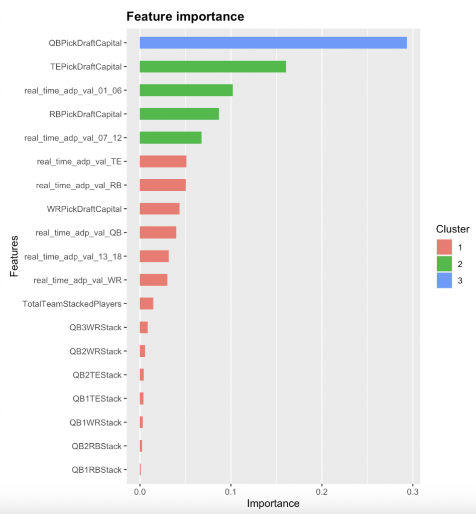
The above visual has some highly-correlated features and low-impact features removed from the actual model we used. 

“Importance” here represents the increase in predictive accuracy of the model when a given variable is included vs. when it is not (e.g., including “QBPickDraftCapital” in the model leads to a huge improvement in the model’s accuracy).

One final note before digging into the results: These models are overfit. While XGBoost can protect against overfitting, we are only dealing with results from one NFL season, which has an incredibly volatile result. This analysis is meant to draw conclusions about what worked (and why) in Best Ball Mania 3, but the volatile nature of that one-season sample means we should not apply everything blindly to Best Ball Mania 4. For example, how much different are last year’s results if Cooper Kupp never gets hurt, if Travis Kelce does get hurt, or if that Week 17 Bills-Bengals game ended up getting played? There are thousands of these small factors that, if changed, would create a massive swing in the results of this tournament.

 

Model Results

It was fascinating pouring over the results of the model. I split up the top 100 teams to glean some characteristics among them and compared them to the 100 teams most closely centered around the 20th percentile (referred to as “20th-percentile teams” from here on out).

Here were some of the more interesting findings:

 

ADP Value (measured by ADP Capital)

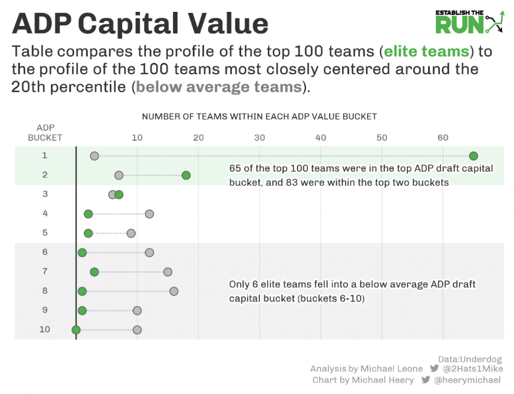
• 65% of all elite teams were in the top ADP capital bucket (only 3% of 20th-percentile teams).
• Only 6% of elite teams had a below-average ADP capital bucket (63% of 20th-percentile teams).

 

WR versus RB Spending

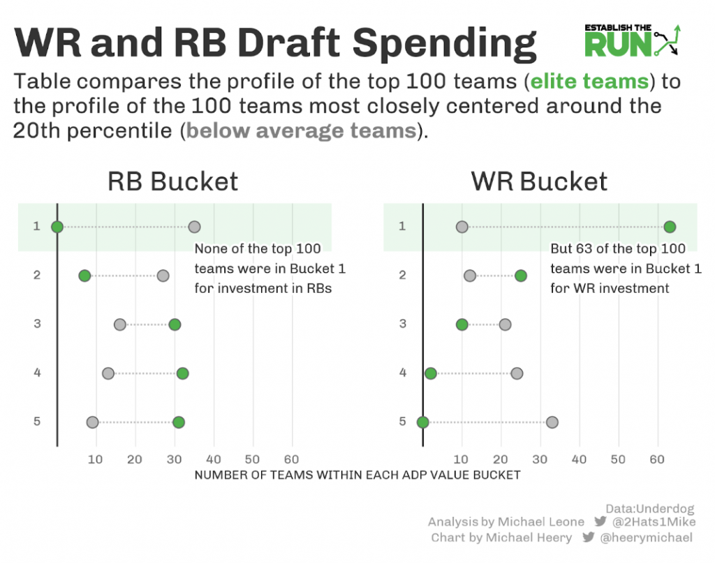
• Elite teams spent way more on WR than 20th-percentile teams.
• Conversely, elite teams spent way less on RBs than 20th-percentile teams.
• Interestingly, RB Buckets 3-5 were represented more or less equally among elite teams, even though we know that in isolation, RB Bucket 5 outperformed RB Bucket 4 and RB Bucket 4 outperformed RB Bucket 3.
• Continuing that thought, it seems RB spending ceased to matter as much among elite teams as long as:
  • They weren’t in Buckets 1 and 2.
  • They still invested heavily in WR.

 

Onesie Positions

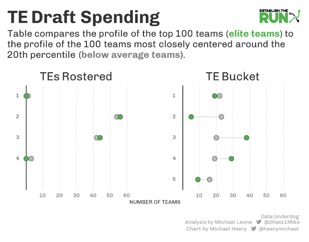
• There was almost no difference between elite and below-average teams in the number of TEs rostered.
• Elite teams more frequently bypassed the second tier of TE spending (Bucket 2), which is perhaps a result of overfitting (Kyle Pitts, Darren Waller, and George Kittle represented a lot of these teams).
• Elite teams were less likely to fully skimp on the position.

 

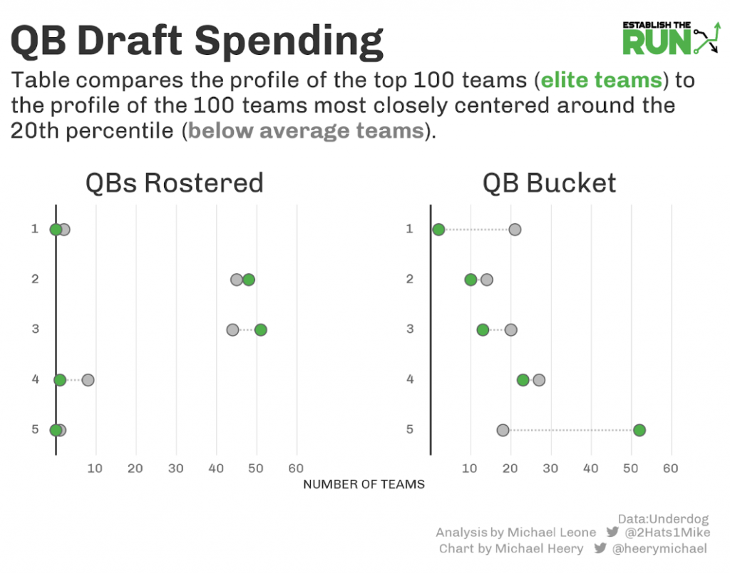
• Both elite and below-average teams rostered two and three QBs at a similar rate.
• This is interesting because the isolated QB analysis suggests that two QBs clearly trump three QBs.
• Similarly, the isolated QB analysis showed that spending in QB Buckets 1 and 2 was most profitable, but the elite teams were way less likely to spend in Bucket 1 and more likely to spend in Bucket 5 (half the teams).
• This is another spot to remind people about overfitting (wouldn’t take this to mean three QBs and little QB spending is a goal for 2023), but it is fascinating how our holistic modeling differs so much from the cohort analysis.

 

Stacking

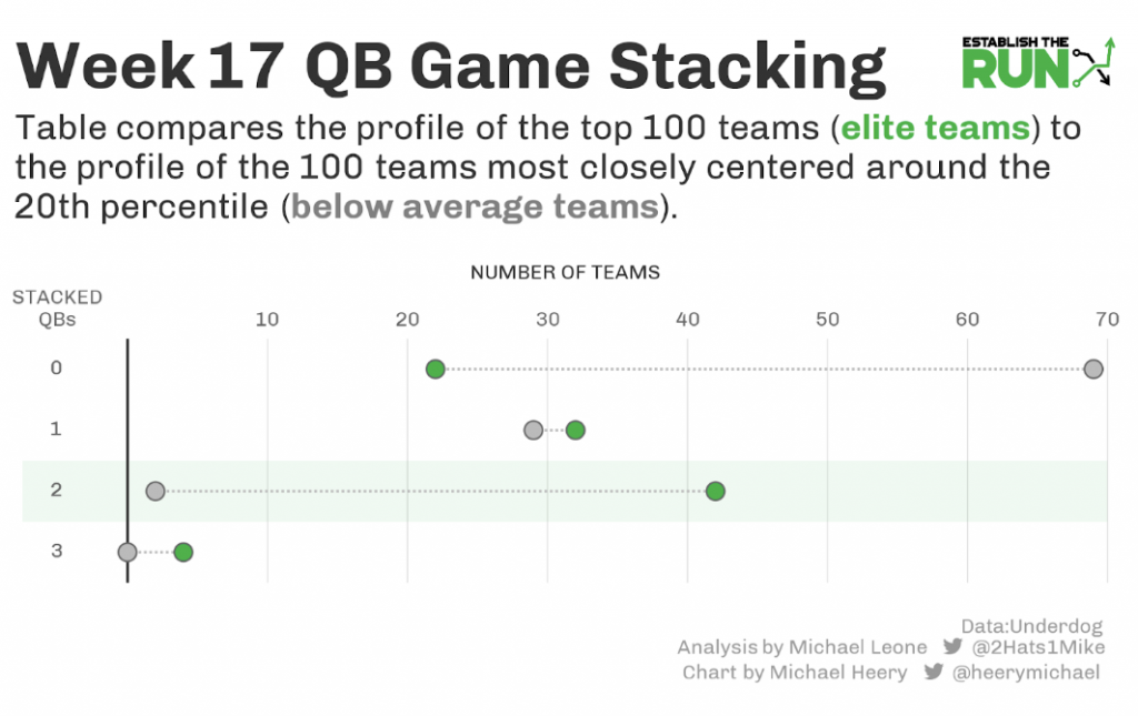
• Unsurprisingly, elite teams game stacked at a massively higher rate than below-average teams.
• While game stacking is clearly important, you were more than twice as likely to find an elite team with zero game stacks than you were to find an elite team with even a bottom 50th-percentile ADP capital.

 

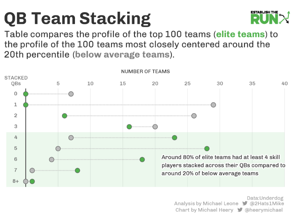
Note that total team-stacked players includes same-team RBs while the number of QBs game-stacked metric does not.

• Once again, correlation is way more present in the elite teams.
• Roughly 80% of elite teams had at least four skill players stacked with one of their QBs (could be spread among multiple QBs).
• Below-average teams were way on the other end of the spectrum, stacking four skill players roughly 20% of the time.

 

Since 100 teams is a pretty small sample, I also reran this analysis looking at the top 1,000 teams and the 1,000 teams most closely centered on the 20th percentile.

• All of the trends stayed the same, with some small magnitude changes, most of which started to better reflect the overall cohort analysis.
• The impact of real-time ADP capital gets reduced a bit. Teams in ADP Capital Bucket 1 dropped from 65% to 45%, and teams with a bottom 50th-percentile ADP capital doubled from 6% to 12%.
• We did see the RB Bucket 5 teams start to get more represented among elite teams, predictably at the expense of RB Bucket 3 teams.
• 2-QB teams were about 60% more likely to be elite teams than 3-QB teams (was split evenly when looking at only 100 teams).
• We still saw a lot of Bucket 5 QB teams, but they dropped from over 50% to 33% with most of that difference being made up in QB Buckets 1 and 2.
• The TE stuff was really similar overall, but we did see a few more TE Bucket 1 teams represented among the elite teams.
• The stacking analysis did not change much.

 

It’s interesting that some of the peculiarities with the above analysis (less QB spending, more 3-QB teams, acceptable RB spending in Bucket 3) directly applied to Kerrane’s winning team.

 

What do elite teams look like?

Here are a few examples among the 10 best overall graded teams by our model. Please keep in mind these grades are meant to represent the strength of a team at the time it was drafted.

 

HyperFragile

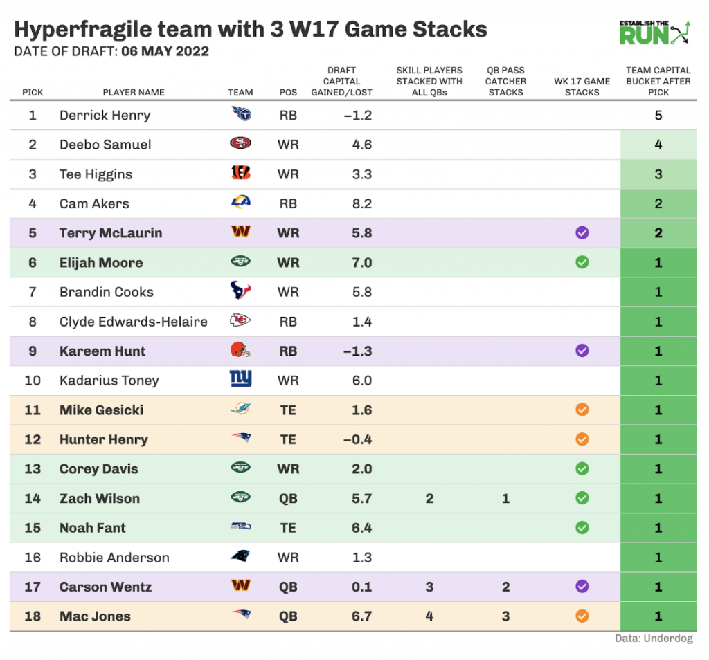
Notes:

• Hyperfragile works when RB spending is not overdone (just four, only two in the first seven rounds) and WR spending is still top-notch.
• The model seems to have an affinity for premium skill-player investment when it comes to the finals model, making room for cheaper but higher-quantity onesie teams to crop up to the top. This team has three QBs and three TEs but minimal total investment in each.
• Personally, this is where I think the model may lack nuance, as I’m not sure there’s enough QB upside to really have this team win.
• Along those same lines, the model is picking up on the impressive stacking power of this team — three separate QB-pass catcher stacks, three Week 17 game stacks, two Week 16 game stacks, and a Week 15 game stack. However, these are pretty cheap stacks. A future version of this model should account for the draft capital invested into the stacks. Cheap stacks are better than no stacks, but this team is probably unfairly credited with a high weekly upside it doesn’t truly possess.
• This team was drafted on May 6. As I noted above, teams drafted earlier underperformed model expectations (days until the start of the season from the draft is a good future variable for us to add). The real-time ADP capital gains were impressive, but the closing line ADP bucket was middle of the pack.

 

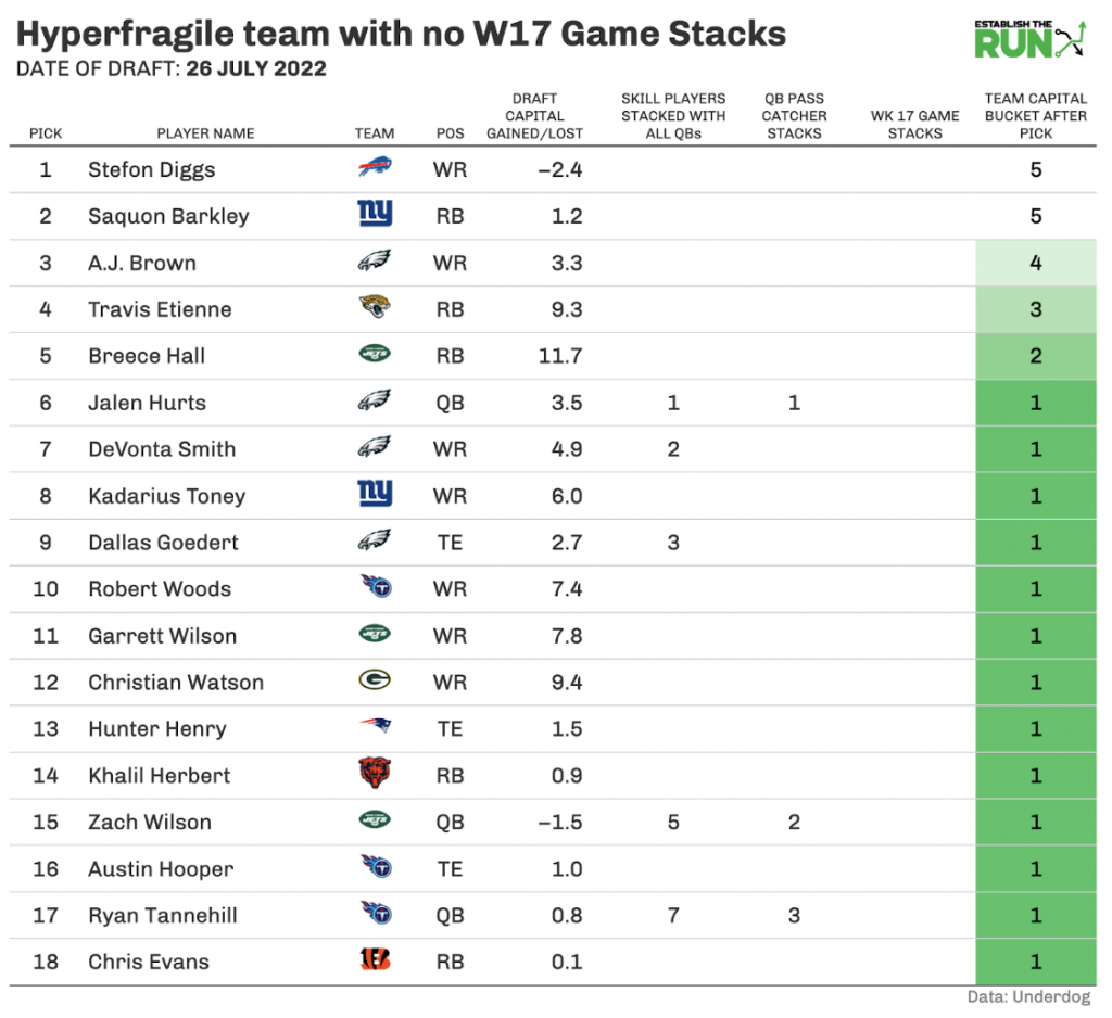
Notes:

• This team had zero Week 17 game stacks, but it did have a game stack in Weeks 15 and 16.
• It had a premium double stack with Jalen Hurts.
• If you view Zach Wilson as an “upside candidate” (we did at ETR last offseason, sigh), you get a pass catcher (Garrett Wilson) and a same-team RB (Breece Hall in Round 5).
• Ryan Tannehill was a token filler stack late.
• This is another of those “RB Bucket 3” teams that still devoted enough firepower to the WR position.
• Being drafted in July, the huge ADP capital gains mostly held. It’s crazy to think of a team in July as being drafted “late”, but this team was drafted much closer to the end of the drafting season than to the beginning.

 

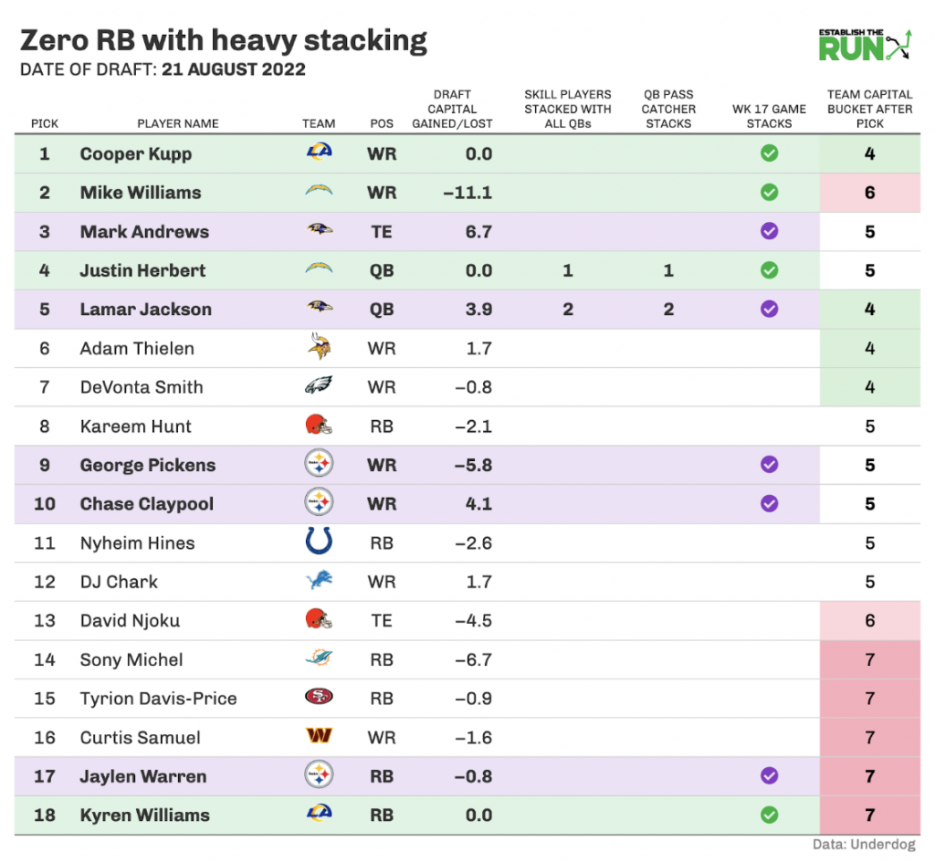
Notes:

• Oddball team in the top 100
  • One of the biggest investments in QB capital among elite teams
  • One of the worst ADP capital buckets among elite teams
• This was a zero RB build with heavy stacking.
• Herbert is single stacked with Mike Williams, but the Week 17 game stack there also includes Cooper Kupp and Kyren Williams.
• Lamar is single stacked with Mark Andrews, but the Week 17 game stack there also includes George Pickens, Chase Claypool, and Jaylen Warren.
• The overinvestment in QB is deemed as tolerable because this team was actually in Bucket 1 of spending at both WR and TE despite those early QB picks (something zero RB allows you to do). There’s a thought experiment in there somewhere about zero RB allowing you to sacrifice ADP value a bit in order to build premium stacks while spending at the onesie positions.

 

Regular-Season Standout

Here’s a team that rated particularly well for the regular season:

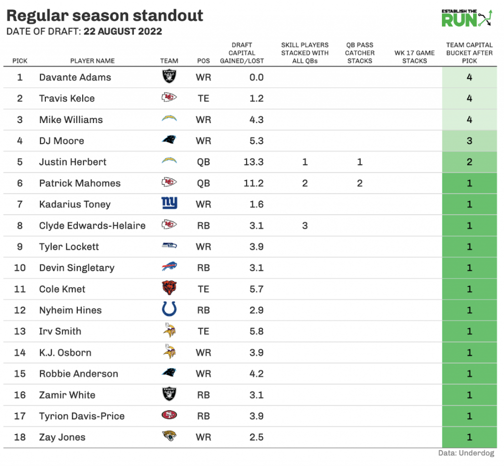
Notes:

• Huge ADP capital gains close to the season
• This is a zero RB team that again allows double-QB investment with an elite TE while only sacrificing a little bit of WR investment (Bucket 2).
• They probably should have replaced a TE with an RB given the start with Kelce.
• Having zero Week 17 or Week 15 game stacks hurts playoff equity and just three total skill players stacked with their QBs does as well (one of which is an RB, so it doesn’t boost the playoff equity much).

 

HyperFragile Playoff/Finals Standout

Here’s a team that rated well specifically for the playoff weeks (individually), particularly in the finals:

Notes:

• True hyperfragile build, three RBs out of the gate and then done
• Is able to still be in Bucket 2 of WR spending:
  • Drafts 11 total
  • Gets positive ADP capital gains on 10 of 11 drafted WRs, so WRs stronger than pure draft capital investment indicates
• 2-QB build with both QBs stacked heavily
• Once again, I think the model is not putting enough stock into QB upside.
• However, it’s important to note that this team stands out with a high finals projected win rate *given the team makes it to the finals in the first place*. This team has just an 11.5% projected regular-season advance prediction, well below that of randomness (16.7%).

 

I hope going through specific teams that our model flagged as elite, either overall, for the regular season, or for the finals, was helpful in visualizing how a good draft comes together. I think the results highlight how various levers working together are important, and you need to be flexible to pull the right ones at the right time.

 

The top areas I’d like to improve in a future version of our model are: 

• training the model on multiple years of data
• accounting for the value and raw investment in team and game stacks
• including “number of days until the NFL season” as a variable for each draft
• making a subjective distinction between low-end QBs with upside vs. without upside

 

One point I’ve made only mildly thus far but I think is important: Player takes matter. If you draft as if you’re right with an early RB you really like or a late-round QB you feel has meaningful upside, you can game the system and shift around how you’re spending your capital to maximize your team’s upside if you are indeed right on that one point. You have to be careful to not take the “draft as if you’re right” mantra too far, leaving yourself unnecessarily fragile in spots, but you should let your intuition (and the ETR rankings if you’re a subscriber) lend you additional upside beyond the strategies that have been outlined in this manifesto.

 

When Best Ball Mania 4 is announced, I’m hopeful that this manifesto can help get you thinking critically about how you should approach your drafts. I think this analysis is flexible enough that you should be able to apply it to Best Ball Mania 4 even though we’re going to see changes in:

• the structure of the contest itself
• the behavior of those we’re drafting against
• a different pool of players and prices available to drafters

 

If you want to jump back to any of the four parts in particular, here are the links to do so:

Introduction
Part 1 – Stacking
Part 2 – ADP Value
Part 3 – Roster Construction
Part 4 – Grading Drafts